Rectangular coordinates
Let's start with the most familiar coordinate system, called rectangular or sometimes rectilinear or Cartesian coordinates. These are the coordinates \( (x,y,z) \) that describe distances along a set of three perpendicular axes. Any choice of three axes will do, as long as they're all mutually perpendicular!
At this point, it's good to introduce vector notation, which will be very helpful in thinking about relating different coordinate systems. We define three unit vectors \( \hat{x}, \hat{y}, \hat{z} \) which point along the corresponding axes. Then we can write any other vector in terms of the unit vectors. For example, the position vector \( \vec{r} \) describes the location of an object relative to the origin:
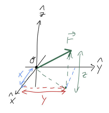
\[ \begin{aligned} \vec{r} = x \hat{x} + y \hat{y} + z \hat{z} \end{aligned} \]
Common alternative names for the unit vectors are \( \hat{i}, \hat{j}, \hat{k} \) and \( \hat{e}_1, \hat{e}_2, \hat{e}_3 \); the latter generic-looking set are sometimes used to describe other coordinate systems, so beware!
(Notation aside: I will use arrows to denote vectors; Taylor uses bold-face, so he would write the vector above as \( \mathbf{r} \). Bold-face is hard to use when you're writing by hand!)
One thing I'll emphasize over and over is keeping track of units (this will save you hours of confusion and many mistakes over the course of your physics career!) Since \( \vec{r} \) has units of distance, and so do the individual lengths \( x,y,z \), we notice that _the unit vectors themselves have no units_ - they just point in a direction.
When we want to refer to components of a vector by name, we'll use a subscript equal to the corresponding unit vector: for example, if \( \vec{v} \) is a velocity, then \( v_x \) is the speed in the x-direction. For the position vector,
\[ \begin{aligned} r_x = x \end{aligned} \]
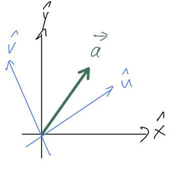
The dot product between two vectors multiplies them together component by component and gives back a number:
\[ \begin{aligned} \vec{a} \cdot \vec{b} = a_x b_x + a_y b_y + a_z b_z \end{aligned} \]
(Some jargon: the dot product is an example of a scalar. A scalar is a quantity that doesn't care about direction; in other words, numbers that aren't vectors are scalars.)
The dot product of a vector with itself gives us the square of its length, just by the Pythagorean theorem:
\[ \begin{aligned} |\vec{r}| = \sqrt{ x^2 + y^2 + z^2} = \sqrt{\vec{r} \cdot \vec{r}} \end{aligned} \]
More notation: paired vertical lines gives absolute value for a regular number, but length for a vector. They're really the same thing, because a vector's length can't be negative, and it's easy to show that \( |-\vec{r}| = |\vec{r}| \). When it isn't ambiguous, I'll usually write this simply as \( r = |\vec{r}| \).
In general, if you go look up some trigonometry formulas, it's not too hard to show that
\[ \begin{aligned} \vec{a} \cdot \vec{b} = ab \cos \theta, \end{aligned} \]
where \( \theta \) is the angle between the two vectors. I won't derive this formula, but I will apply one other concept that I'll emphasize over and over, which is checking limits and special cases (another technique to save you from hours of frustration!) First special case: if \( \vec{b} = \vec{a} \), then the angle \( \theta \) is obviously zero, and we recover the formula \( \vec{a} \cdot \vec{a} = |\vec{a}|^2 \) from above. Our check is successful!
Another interesting limit is when \( \theta = 90^\circ \): the formula tells us that the dot product should be \( ab \cos 90^\circ = 0 \). If we pick our coordinates axes so that \( \vec{a} = a \hat{x} \) and \( \vec{b} = b \hat{y} \), for example, then it's easy to confirm this from the definition. So this check passes too.
A natural question you might ask is: what if I've already picked my coordinate axes, and my vectors point in different directions? Why does the argument above still work? A really important point to remember is that vectors exist independent of our choice of coordinates. Mathematically, this is true by definition: obviously in physics, it had better be true, because a block sliding down a ramp only has a single velocity vector even if you and I measure it differently.
Since \( \vec{a} \cdot \vec{b} \) only depends on the vectors and not on any components, it is coordinate-independent, and we can always set up the special coordinates described above to figure out the dot product when \( \theta = 90^\circ \).
We emphasized that unit vectors like \( \hat{x} \) just point in a direction: they carry no units and their length doesn't change. Using the dot product, we can define a unit vector pointing in the direction of any vector by dividing its length out:
\[ \begin{aligned} \hat{a} = \frac{1}{\sqrt{(\vec{a} \cdot \vec{a})}} \vec{a}. \end{aligned} \]
or using our informal notation for the length and inverting, \( \vec{a} = a \hat{a} \). As another example, we can write the position vector as \( \vec{r} = r \hat{r} \).
The other important vector product to know is the cross product, \( \vec{a} \times \vec{b} \). This gives us another vector instead of a number, and in particular \( \vec{a} \times \vec{b} \) by definition is perpendicular to both \( \vec{a} \) and \( \vec{b} \). The magnitude of the cross product is
\[ \begin{aligned} |\vec{a} \times \vec{b}| = ab \sin \theta \end{aligned} \]
behaving in the opposite way to the dot product; in particular, notice that \( |\vec{a} \times \vec{a}| \) is always zero.
Now, given two different vectors \( \vec{a} \) and \( \vec{b} \), there is a unique plane containing both of them; the direction of the cross product \( \vec{a} \times \vec{b} \) is then perpendicular to that plane. However, this isn't quite enough information, because \( -\vec{a} \times \vec{b} \) is also perpendicular to the plane!
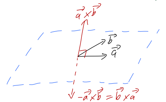
Deciding which of these two vectors to call the positive cross product is a choice of convention - which means it's an arbitrary choice that we can make once, but then we have to keep that choice consistent. We will follow the standard physics convention, which is the right-hand rule: if you hold out your right hand with the thumb pointing in the direction of \( \vec{A} \) and your fingers in the direction of \( \vec{B} \), then your palm points in the direction of \( \vec{A} \times \vec{B} \). Try it with my diagram above!
The right-hand rule also fixes an ambiguity in our rectangular coordinates, which is that we could have picked either of these sets of axes:
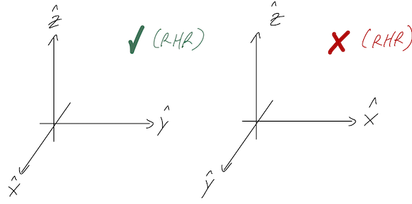
We always define our rectangular coordinates so that positive \( \hat{z} \) is a right-hand rule cross product of \( \hat{x} \) with \( \hat{y} \). In other words, the directions of our rectangular unit vectors always satisfy:
\[ \begin{aligned} \hat{x} \times \hat{y} = \hat{z} \\ \hat{y} \times \hat{z} = \hat{x} \\ \hat{z} \times \hat{x} = \hat{y}. \end{aligned} \]
This is only one choice of convention, and not three; the first equation actually forces the other two to be true. An easy way to remember all three of these at once is to notice that they are all cyclic permutations: if you shift every vector to the left one spot, wrapping back around to the right at the left end, then you get the next formula.
There is a general, mechanical formula for the cross product in rectangular components, using a three-by-three matrix determinant:
\[ \begin{aligned} \vec{a} \times \vec{b} = \left|\begin{array}{ccc} \hat{x}&\hat{y}&\hat{z}\\ a_x&a_y&a_z\\ b_x&b_y&b_z\end{array}\right| \\ = (a_y b_z - a_z b_y) \hat{x} - (a_x b_z - a_z b_x) \hat{y} + (a_x b_y - a_y b_x) \hat{z}. \end{aligned} \]
We will use this rarely if at all this semester, so don't worry about memorizing it at this point; it's more important to know the general formulas above for length and direction of a cross product.
Cylindrical coordinates
I'll do cylindrical coordinates next, because they only swap out two out of three coordinates from Cartesian coordinates: \( \hat{z} \) is kept the same. Ignoring the \( z \)-direction, we want to swap out the other two coordinates \( (x,y) \) for 2-d polar coordinates:
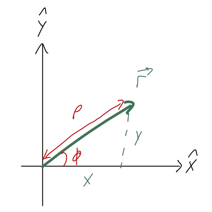
As we can read off the sketch, the relationship between the coordinates is
\[ \begin{aligned} x = \rho \cos \phi \\ y = \rho \sin \phi \end{aligned} \]
or going backwards,
\[ \begin{aligned} \rho = \sqrt{x^2 + y^2} \\ \tan \phi = \frac{y}{x}. \end{aligned} \]
A word of warning about this last formula: you might be tempted to just use an inverse function to "simplify" it and write \( \phi = \tan^{-1} (y/x) \). The problem with this will be obvious if we plot the \( \tan^{-1} \) function:
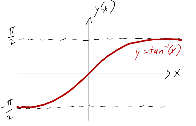
The range of \( \tan^{-1} \), i.e. its set of possible output values, is \( (-\pi/2, \pi/2) \). But this only covers half of the plane! The issue is that if we reflect a point from \( (x,y) \rightarrow (-x,-y) \), the value of the ratio \( y/x \) doesn't change: in terms of angles, \( \tan (\phi + \pi) = \tan \phi \). So if you use the ratio \( y/x \) to find what the coordinate \( \phi \) is, double-check what quadrant your point is supposed to be in!
(Aside: if you're doing this numerically, it's not hard to write a computer program that will use \( \tan^{-1} \) and then check the signs and add \( \pi \) if needed. However, the program needs to know both \( x \) and \( y \) separately. In Mathematica, if you give two numbers i.e. ArcTan[x,y], it gives you exactly this corrected result for \( \phi \). In other programming languages, the 'quadrant-aware' version of the function is usually called arctan2.)
Note: Taylor does something I think is confusing, which is to use \( r \) instead of \( \rho \) if he's in two dimensions. I'll always use \( \rho \) for the polar radius, keeping \( r \) for the three-dimensional position vector, i.e. distance to the origin. If \( z=0 \), then these are the same.
If we want to do integrals in cylindrical coordinates, we need the volume element dV. You should be able to readily show from the equations above, starting from the rectangular \( dV = dx dy dz \), that
\[ \begin{aligned} dV = \rho\ d\rho\ d\phi\ dz. \end{aligned} \]
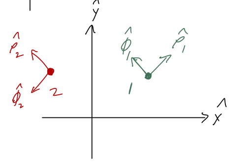
On to the unit vectors. Remember that the idea of a coordinate unit vector is that it points in the direction in which that coordinate increases. But now, if we choose a couple of points and identify \( \hat{\rho} \) and \( \hat{\phi} \), it's easy to see that we have a new complication: the directions \( \hat{\rho} \) and \( \hat{\phi} \) depend on what point we are asking about!
We can do a bit of trigonometry on any given point and easily show the general relationship
\[ \begin{aligned} \hat{\rho} = \cos \phi \hat{x} + \sin \phi \hat{y} \\ \hat{\phi} = -\sin \phi \hat{x} + \cos \phi \hat{y} \end{aligned} \]
The way in which they depend on our coordinates isn't so bad: their directions just change with the angle \( \hat{\phi} \).
By the way, there's another way to derive these relationships. When we take the derivative of a vector \( \vec{v} \) with respect to some other variable \( s \), the new vector \( d\vec{v}/ds \) gives us both the rate and the direction of change with respect to \( s \). So converting our words "unit vector pointing in the direction in which a coordinate increases" into equations,
\[ \begin{aligned} \hat{\rho} = \frac{d\vec{r}/d\rho}{|d\vec{r}/d\rho|} \\ \hat{\phi} = \frac{d\vec{r}/d\phi}{|d\vec{r}/d\phi|} \end{aligned} \]
We stopped with an exercise: try using these formulas yourself with our coordinate definitions above, to re-derive the unit vectors \( \hat{\rho} \) and \( \hat{\phi} \) in terms of \( \hat{x} \) and \( \hat{y} \). Next time, we'll pick up there!