We started by finishing the exercise from last time:
Exercise: Polar unit vectors as rates of change
Derive the unit vectors \( \hat{\rho} \) and \( \hat{\phi} \) in terms of Cartesian unit vectors \( \hat{x}, \hat{y} \) by taking derivatives of \( \vec{r} \).
Since this is the first exercise, let me explain a bit. These are meant to be interactive examples: in lecture, I will pause here and give you a few minutes to work on it yourself. After a few minutes, I'll finish the example and take questions.
IMPORTANT: you do not have to finish the exercise in the time I give you! It's only important that you start to think about how you would set things up and work through the example. If you run out of time or get stuck, it may be helpful for you to go over it on your own after lecture.
If you're reading the lecture notes afterwards and haven't done the exercise yet, now is a great time to stop reading, go try it yourself, and then come back and read the answer.
Solution: We start by writing \( \vec{r} \) out in Cartesian components, ignoring \( \hat{z} \):
\[ \begin{aligned} \vec{r} = x\hat{x} + y\hat{y} \end{aligned} \]
Next, we substitute in the formulas for \( x \) and \( y \) in terms of cylindrical coordinates:
\[ \begin{aligned} \vec{r} = \rho \cos \phi \hat{x} + \rho \sin \phi \hat{y} \end{aligned} \]
Now we can take derivatives, remembering that the derivative of a vector is still a vector:
\[ \begin{aligned} \frac{d\vec{r}}{d\rho} = \cos \phi \hat{x} + \sin \phi \hat{y} \end{aligned} \]
and
\[ \begin{aligned} \frac{d\vec{r}}{d\phi} = -\rho \sin \phi \hat{x} + \rho \cos \phi \hat{y} \end{aligned} \]
These are the correct directions for \( \hat{\rho} \) and \( \hat{\phi} \) already; to make them unit vectors, we just have to normalize. It's easy to show that \( d\vec{r}/d\rho \) is already a unit vector, while the length of the other vector is
\[ \begin{aligned} \left| \frac{d\vec{r}}{d\phi} \right| = \sqrt{\rho^2 (\sin^2 \phi + \cos^2\phi)} = \rho. \end{aligned} \]
So finally, we have
\[ \begin{aligned} \hat{\rho} = \frac{d\vec{r}/d\rho}{|d\vec{r}/d\rho|} = \cos \phi \hat{x} + \sin \phi \hat{y} \\ \hat{\phi} = \frac{d\vec{r}/d\phi}{|d\vec{r}/d\phi|} = -\sin \phi \hat{x} + \cos \phi \hat{y} \end{aligned} \]
matching the result above.
Since I mentioned it, the last thing I'll point out for cylindrical coordinates is that we can use what we've defined above to show that the position vector here becomes
\[ \begin{aligned} \vec{r} = \rho \hat{\rho} + z \hat{z}. \end{aligned} \]
Notice that there is no \( \hat{\phi} \) component! (Draw a picture, or look at some of the above, to convince yourself that this makes sense.) If you are ever tempted to add a \( \phi \hat{\phi} \) term, you should be stopped by noticing it has the wrong units; \( \vec{r} \) should have units of distance, but \( \phi \) is unitless and so is \( \hat{\phi} \), so something is wrong.
Spherical coordinates
In spherical coordinates, we adopt \( r \) itself as one of our coordinates, in combination with two angles that let us rotate around to any point in space. We keep the angle \( \phi \) in the x-y plane, and add the angle \( \theta \) which is taken from the positive \( \hat{z} \)-axis:
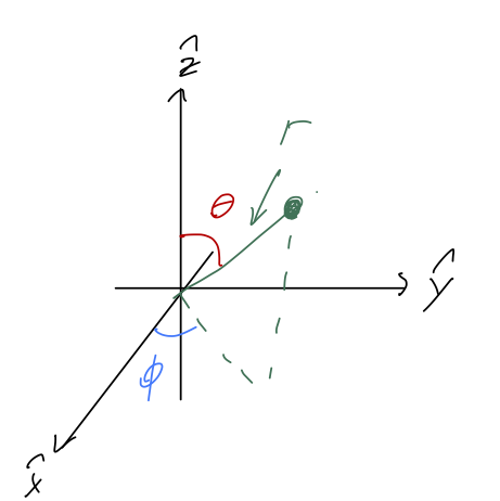
(Confusingly, \( \theta \) is usually called the "polar angle", thinking of the z-axis as the "pole". In this case, \( \phi \) is called the "azimuthal angle". See Taylor, p.135.)
Important note: these are the physics conventions for what to call these angles. Mathematicians tend to prefer the opposite choice, using \( \theta \) as the azimuthal angle and \( \phi \) the polar. Math books (and some physics texts) will also use \( \rho \) for the spherical distance and \( r \) the polar distance. Be very careful when looking at other resources!
The relationship between spherical and cylindrical coordinates is actually relatively simple to work out, as we can see by looking at a cross-section containing both \( \vec{r} \) and \( \hat{z} \):
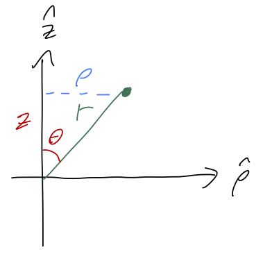
It's easy to see from the sketch that
\[ \begin{aligned} z = r \cos \theta \\ \rho = r \sin \theta \end{aligned} \]
We can then take this and plug in one more step to get the formulas for rectangular coordinates:
\[ \begin{aligned} x = r \sin \theta \cos \phi \\ y = r \sin \theta \sin \phi \\ z = r \cos \theta \end{aligned} \]
If you forget exactly where the sine and cosines go in this expression, I find it's easiest to think about converting from cylindrical coordinates. As before, we can use this to find the volume element for doing integrals:
\[ \begin{aligned} dV = r^2 \sin \theta\ dr\ d\theta\ d\phi. \end{aligned} \]
When doing an integral, it's important to set up the limits of integration properly. This sometimes requires a bit of thought for the two angular coordinates: one angle is ambiguous (e.g. \( \phi \) and \( \phi+2\pi \) are the same point), and having two angles introduces some new ambguities.
In particular, if we start by letting the x-y planar angle \( \phi \) run from 0 to \( 2\pi \), just like in two dimensions, then you can convince yourself from the diagram above that the other angle \( \theta \) has to run from 0 to \( \pi \). (Basically, this is because \( (\phi, -\theta) \) is the same point as \( (\phi + \pi, +\theta) \).)
We could find results for the unit vectors in spherical coordinates \( \hat{\rho}, \hat{\theta}, \hat{\phi} \) in terms of the Cartesian unit vectors, but we're not going to be doing vector calculus in these coordinates for a while, so I'll put this off for now - it's a bit messy compared to cylindrical.
Motion and Newton's laws
Now that we've set up our math basics, let's turn back to physics, starting with Newton's laws of motion. Taylor discusses some fundamentals about defining mass and force, but I'll let you read that on your own. First, let's remind ourselves what Newton's three laws of motion are in words:
- In the absence of forces, an object moves with constant velocity.
- An object of mass \( m \) subject to a net force will accelerate according to the relation
\[ \begin{aligned} \vec{F} = m \vec{a}. \end{aligned} \]
- If object 1 exerts a force on object 2, there is an equal and opposite force exerts on object 2 by object 1,
\[ \begin{aligned} \vec{F}_{12} = -\vec{F}_{21}. \end{aligned} \]
In our modern understanding, the first law is more or less redundant, because the second law immediately tells us that if \( \vec{F} = 0 \), then \( \vec{a} = 0 \); since \( \vec{a} = d\vec{v}/dt \), no acceleration means constant velocity. (This isn't quite true, because you can think of the first law as something to check to make sure you're in an inertial frame where the second law will hold; see the discussion in Taylor, chapter 1. More on inertial frames in a bit.)
We mentioned vector derivatives before, but let's talk a bit more about them, and time derivatives specifically. Backing up a step, the velocity vector is the time derivative of the position vector,
\[ \begin{aligned} \vec{v} = \frac{d\vec{r}}{dt} \end{aligned} \]
We can think about the meaning of this expression by unpacking it using unit vectors and the product rule:
\[ \begin{aligned} \frac{d}{dt} \vec{r} = \frac{d}{dt} \left( x \hat{x} + y \hat{y} + z \hat{z} \right) \\ = \frac{dx}{dt} \hat{x} + \frac{dy}{dt} \hat{y} + \frac{dz}{dt} \hat{z} \\ = \dot{x} \hat{x} + \dot{y} \hat{y} + \dot{z} \hat{z}. \end{aligned} \]
Here I introduce some new notation, since we'll be taking lots and lots of time derivatives: a dot over a quantity indicates acting on it with \( d/dt \). This applies both to scalars and vectors, so for example we can write \( \vec{v} = \dot{\vec{r}} \). Finally, multiple dots can be used for multiple derivatives, so Newton's second law can be written out as
\[ \begin{aligned} \vec{F} = m \vec{a} = m \frac{d^2 \vec{r}}{dt^2} = m \ddot{\vec{r}}. \end{aligned} \]
Since we just looked at the decomposition of \( \dot{\vec{r}} \) in Cartesian coordinates, let's look at Newton's second law in the same coordinates. Taking another time derivative will just give us double-dots instead of single-dots on the right side of the equation, so we have:
\[ \begin{aligned} F_x \hat{x} + F_y \hat{y} + F_z \hat{z} = m \left(\ddot{x} \hat{x} + \ddot{y} \hat{y} + \ddot{z} \hat{z} \right) \end{aligned} \]
This is, in fact, just three separate copies of the same equation, one for each direction:
\[ \begin{aligned} F_x = m\ddot{x} \\ F_y = m\ddot{y} \\ F_z = m\ddot{z} \end{aligned} \]
Although it's usually taken as obvious, you might ask at this point why we're allowed to break one equation up into three. Because this is a vector equation, and two vectors will only be equal if all of their components are equal, we can just check one component at a time. Of course, that means that we have a system of equations, which must all be true at once. These equations are collectively known as the equations of motion, because if we solve them, we know the answer for \( \vec{r}(t) \) - we know what the motion of the system will look like over time.
Example: block on a ramp and coordinate choices
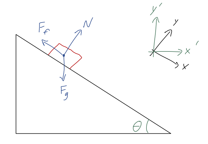
Taylor does this as his example 1.1, but he takes his \( x \)-axis to be parallel to the ramp. To get used to comparing different coordinate systems, I'll instead set my \( y \)-axis to be in the direction of gravity - I'll call this the \( y' \) axis. As Taylor points out, this will make things slightly more complicated, but it's not too bad.
We'll treat this as a two-dimensional problem, as indicated, which just means that we ignore the \( z \) coordinate. (This is valid because of Newton's first law: if there are no \( z \)-direction forces, then there is no interesting \( z \)-direction motion at all.) The forces split into components are, using the often-convenient notation that \( \vec{F} = (F_x, F_y) \):
\[ \begin{aligned} \vec{N} = (N \sin \theta, N \cos \theta) \\ \vec{F}_f = (-F_f \cos \theta, F_f \sin \theta) \\ \vec{F}_g = (0, -mg) \end{aligned} \]
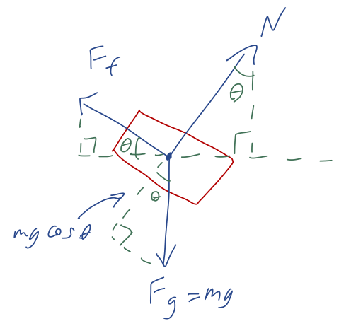
(if where I put the \( \theta \)'s in my diagram isn't obvious to you, draw more parallel lines in and use right triangles to identify which angles are \( \theta \) and which are \( 90^\circ - \theta \).)
Now, we know that the normal force \( N \) is equal and opposite to the magnitude of all other forces acting perpendicular to the surface of the ramp. We can actually write this statement out using dot products:
\[ \begin{aligned} N = |\vec{F}_f \cdot \hat{N} + \vec{F}_g \cdot \hat{N}| \end{aligned} \]
Since we have all the vectors in components above, and since it's easy to see that \( \hat{N} = (\sin \theta, \cos \theta) \), we can easily work out the dot products:
\[ \begin{aligned} \vec{F}_f \cdot \hat{N} = -F_f \sin \theta \cos \theta + F_f \cos \theta \sin \theta = 0 \\ \vec{F}_g \cdot \hat{N} = -mg \cos \theta \end{aligned} \]
and so
\[ \begin{aligned} N = mg \cos \theta. \end{aligned} \]
Notice that although we used algebra to find the answer, this would have been easy to work out geometrically too:
The second thing we know is that the magnitude of the frictional force is related to the normal force:
\[ \begin{aligned} F_f = \mu N = \mu mg \cos \theta \end{aligned} \]
Plugging back in, then, we have the net forces in the \( x' \) and \( y' \) directions:
\[ \begin{aligned} \vec{F}_{\rm net} = \vec{N} + \vec{F}_f + \vec{F}_g \\ = \left(N \sin \theta - F_f \cos \theta \right) \hat{x}' + \left(N \cos \theta + F_f \sin \theta - mg \right) \hat{y}' \\ = mg \left( \cos \theta \sin \theta - \mu \cos^2 \theta \right) \hat{x}' + mg \left(\cos^2 \theta + \mu \cos \theta \sin \theta - 1 \right) \hat{y}' \end{aligned} \]
This looks a little messy, but let's keep going. Now that we have the net force, we can solve for the accelerations using \( \vec{F}_{\rm net} = m \ddot{\vec{r}} \), which gives us two equations looking at each component (and cancelling off the mass):
\[ \begin{aligned} \ddot{x}' = g \cos \theta (\sin \theta - \mu \cos \theta) \\ \ddot{y}' = -g (1 - \cos^2 \theta - \mu \sin \theta \cos \theta) \\ = -g \sin \theta (\sin \theta - \mu \cos \theta) \end{aligned} \]
where I've used a trig identity to simplify the last line; now the \( x' \) and \( y' \) equations look very similar.
Next time, we'll finish our solution and check against Taylor.