Now that we've reviewed both Newton's laws and curvilinear coordinate systems, let's have a closer look at what happens when we put the two together. We'll focus mainly on cylindrical coordinates, which will show the important features; spherical is more complicated but not really different.
Remember that one of the nice things about Newton's laws in Cartesian coordinates is that they split apart into three separate equations for the \( x,y,z \) directions. Let's remind ourselves why: Newton's second law reads
\[ \begin{aligned} \vec{F} = m\ddot{\vec{r}} \\ F_x \hat{x} + F_y \hat{y} + F_z \hat{z} = m \frac{d^2}{dt^2} \left( x \hat{x} + y \hat{y} + z\hat{z} \right) \end{aligned} \]
and then acting with the time derivatives and matching components, we read off the individual equations \( F_x = m\ddot{x} \) and so on.
Now, we can do the same thing in cylindrical coordinates, using our results from above:
\[ \begin{aligned} F_\rho \hat{\rho} + F_\phi \hat{\phi} + F_z \hat{z} = m \frac{d^2}{dt^2} \left( \rho \hat{\rho} + z \hat{z} \right) \end{aligned} \]
You might be tempted to just starting matching terms again and conclude that \( F_\rho \stackrel{?}{=} m\ddot{\rho} \). But there's an immediate problem, which is that there doesn't seem to be a \( \hat{\phi} \) term on the right-hand side! Does this mean that \( F_\phi \) is just irrelevant, no matter how large the force is? (That seems like a strange conclusion...)
The resolution to this problem is that the simple argument above is ignoring some of the time dependence. We can see this by drawing two different vectors \( \vec{r}_1 \) and \( \vec{r}_2 \), and noting the directions of the unit vectors:
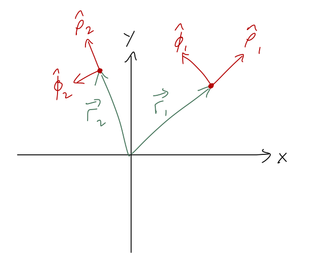
As we noted before, the direction of the cylindrical unit vectors is different for \( \vec{r}_1 \) and \( \vec{r}_2 \). But in the context of mechanics, \( \vec{r}_2 \) could represent a time-evolved version of \( \vec{r}_1 \) for some system, i.e. \( \vec{r}_1 = \vec{r}(t_1) \) and \( \vec{r}_2 = \vec{r}(t_2) \). If so, then it's obvious that the unit vectors \( \hat{\rho} \) and \( \hat{\phi} \) themselves must be time-dependent.
Exercise: time dependence of cylindrical unit vectors
Find the first derivative \( \ d\hat{\rho}/dt \) (and if you have time, \( d\hat{\phi}/dt \).) Express your answer in terms of cylindrical unit vectors.
Another exercise, so if you're reading along, give this a try before you continue. You can do this either with geometry or with algebra...
If you look at Taylor, he'll show you a nice geometric way to find the time derivatives. Instead of repeating him, I'll do it with algebra instead. Remember that we previously found these expressions for the cylindrical unit vectors:
\[ \begin{aligned} \hat{\rho} = \frac{d\vec{r}/d\rho}{|d\vec{r}/d\rho|} = \cos \phi \hat{x} + \sin \phi \hat{y} \\ \hat{\phi} = \frac{d\vec{r}/d\phi}{|d\vec{r}/d\phi|} = -\sin \phi \hat{x} + \cos \phi \hat{y} \end{aligned} \]
Now we can just take time derivatives explicitly, using the fact that \( \hat{x} \) and \( \hat{y} \) are time-independent. Starting with the radial direction,
\[ \begin{aligned} \frac{d\hat{\rho}}{dt} = -\dot{\phi} \sin \phi \hat{x} + \dot{\phi} \cos \phi \hat{y} \\ = \dot{\phi} \hat{\phi}, \end{aligned} \]
recognizing the form of the other unit vector and substituting it back in. Similarly, it's easy to show that
\[ \begin{aligned} \frac{d\hat{\phi}}{dt} = -\dot{\phi} \hat{\rho}. \end{aligned} \]
Now let's go back to Newton's second law and expand out the right-hand side. I'll ignore the \( z\hat{z} \) piece because it's the same as in Cartesian coordinates. What we need is, going slowly:
\[ \begin{aligned} \frac{d^2}{dt^2} \left( \rho \hat{\rho} \right) = \frac{d}{dt} \left( \dot{\rho} \hat{\rho} + \rho \frac{d\hat{\rho}}{dt} \right) \\ = \frac{d}{dt} \left( \dot{\rho} \hat{\rho} + \rho \dot{\phi} \hat{\phi} \right) \\ = \ddot{\rho} \hat{\rho} + \dot{\rho} \frac{d\hat{\rho}}{dt} + (\dot{\rho} \dot{\phi} + \rho \ddot{\phi}) \hat{\phi} + \rho \dot{\phi} \frac{d\hat{\phi}}{dt} \\ = \ddot{\rho} \hat{\rho} + \dot{\rho} \dot{\phi} \hat{\phi} + (\dot{\rho} \dot{\phi} + \rho \ddot{\phi}) \hat{\phi} - \rho \dot{\phi}^2 \hat{\rho} \\ = (\ddot{\rho} - \rho \dot{\phi}^2) \hat{\rho} + (\rho \ddot{\phi} + 2 \dot{\rho} \dot{\phi}) \hat{\phi} \end{aligned} \]
gathering together terms at the end. Putting this back into Newton's second law, we find the equations for the other two components:
\[ \begin{aligned} F_\rho = m(\ddot{\rho} - \rho \dot{\phi}^2) \\ F_\phi = m(\rho \ddot{\phi} + 2\dot{\rho} \dot{\phi}) \end{aligned} \]
The good news is that we now have dependence on all three coordinates, and on all three components of the force. The bad news is that this is going to give much more complicated differential equations for us to solve! (Attacking them directly, using the alternative Lagrangian formulation, is something you'll come back to next semester.)
However, there are specific problems where cylindrical coordinates are the best choice even for solving with Newton's laws. A good example is a simple pendulum:
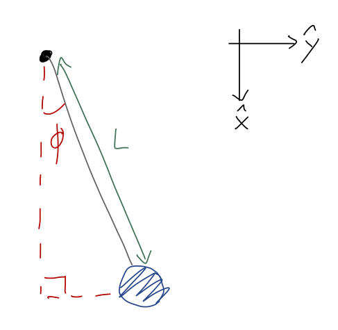
Note that I've turned the coordinates around a bit compared to how we usually draw them; this is so that I can identify the angle \( \phi = 0 \) with the lowest point of the pendulum. (Again, physical intution: we know that hanging straight down is a special point because the pendulum won't move if we start it there. So we anticipate the answer will be a bit simpler with these coordinates.)
For the pendulum, the cylindrical radius is fixed to the length of the string, \( \rho = L \). This means that any time derivatives of \( \rho \) vanish, leaving us with the equations
\[ \begin{aligned} F_\rho = -mL \dot{\phi}^2 \\ F_\phi = mL \ddot{\phi} \end{aligned} \]
Notice, by the way, that if we were studying purely circular motion (e.g. the pendulum is being spun around on a flat surface instead of hanging vertically), we would have \( \dot{\phi} = v/L \), and the first equation becomes
\[ \begin{aligned} F_\rho = -mL \left( \frac{v}{L} \right)^2 = -m\frac{v^2}{L} \end{aligned} \]
which is the familiar equation for centripetal force. (By assumption of circular motion, the angular speed \( \dot{\phi} \) is constant, so the second equation is just \( F_\phi = 0 \).)
Back to the more general case of a pendulum. We should draw a free-body diagram:
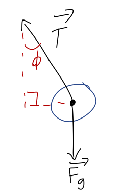
One of the nice things about using cylindrical coordinates is immediately obvious: the tension is always in the radial direction, so we have
\[ \begin{aligned} \vec{T} = -T \hat{\rho} \end{aligned} \]
regardless of where the pendulum is. As for gravity, we will need to decompose it into radial and tangential pieces. This time I'll do it the geometric way, but note that you can also start with \( F_g = -mg\hat{y} \) and use algebra as an alternative way to convert. (Try it out if you're not comfortable with vector algebra yet!) Let's draw angles onto our free-body diagram and identify the unit-vector directions:
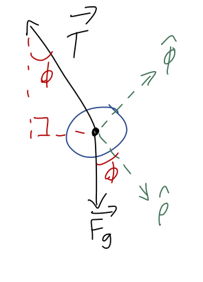
From the sketch, we readily find that
\[ \begin{aligned} \vec{F}_g = mg \cos \phi \hat{\rho} - mg \sin \phi \hat{\phi} \end{aligned} \]
Now we can plug back in to Newton's laws in cylindrical components. Combining the radial forces, the first equation reads
\[ \begin{aligned} mg \cos \phi - T = -mL \dot{\phi}^2 \end{aligned} \]
and the second is
\[ \begin{aligned} -mg \sin \phi = mL \ddot{\phi}. \end{aligned} \]
To solve for the motion, we can completely ignore the first equation, because it contains the unknown tension force \( T \). (If we care about the tension, like if we know our string has a max tension and we want to predict whether it will break, we can go back and check at the end once we know \( \phi(t) \).) The second equation simplifies slightly to:
\[ \begin{aligned} \ddot{\phi} = -\frac{g}{L} \sin \phi. \end{aligned} \]
Let's check units, always a good practice: \( \phi \) is dimensionless, \( g \) has units of \( m/s^2 \), and \( L \) has units of \( m \), so we have \( 1/s^2 \) on the right. This matches the left exactly, because \( d/dt \) itself has units of \( 1/s \). (If this isn't clear to you, think about the basic definition of a derivative: \( du/dt \) comes from the infinitesmal limit of \( \Delta u / \Delta t \), and the units of \( \Delta t \) are clearly the same as the units of \( t \).)
In this case both sides depend on the unknown \( \phi \), so we can't just integrate with respect to time. In fact, this is actually a surprisingly hard differential equation to solve, for such a simple system! There is no analytic solution in terms of elementary functions in general, but we can find an approximate solution: if we assume the angle \( \phi \) is always small (the 'small-angle approximation'), then we can Taylor expand the right-hand side about \( \phi=0 \),
\[ \begin{aligned} \sin \phi \approx \phi\ + ... \end{aligned} \]
giving the simpler equation
\[ \begin{aligned} \ddot{\phi} = -\frac{g}{L} \phi. \end{aligned} \]
This still depends on \( \phi \) on both sides, but it has a relatively simple general solution, of the form
\[ \begin{aligned} \phi(t) = A \sin (\omega t) + B \cos (\omega t) \end{aligned} \]
where \( \omega = \sqrt{g/L} \). At this point, we're not ready to study how to get that general solution yet, but it's easy for you to plug it back in and check that it works.
We're starting to see that there are examples of equations of motion where the forces depend on coordinates, and we can't just solve by simply integrating. In fact, this is a great point for us to go back to math, and start to study the more general theory of differential equations.
Ordinary differential equations
As we've started to see, solving equations of motion requires the ability to deal with more general classes of differential equations. Let's start to think about the general theory of differential equations and how to solve them.
Let's start with some vocabulary. An ordinary differential equation, or "ODE", is one that contains no partial derivatives (if it does have partial derivatives, it's a partial differential equation, or "PDE".) Newtonian mechanics problems are always ODEs, because we only have derivatives with respect to time in the second law.
Next on the list of classification terms is order, which refers to the highest number of derivatives that appear on a single term at once. The simplest possibility is first-order, which has at most one derivative. Examples of first-order equations are
\[ \begin{aligned} \frac{dy}{dx} = -y \\ \frac{dr}{dt} + r * \cos(t) = \pi \\ \exp \left( \frac{du}{dx} \right) - u/x^4 + \sin(x) = 0 \end{aligned} \]
Newton's second law \( \vec{F} = m\ddot{\vec{r}} \) is a second-order equation, due to the two time derivatives.
Now, a very important fact about differential equations is that their solutions alone are not unique; we need more information to find a complete solution. As a simple example, consider the equation
\[ \begin{aligned} \frac{dy}{dx} = 2x \end{aligned} \]
You can probably guess right away that the function \( y(x) = x^2 \) satisfies this equation. But so does \( y(x) = x^2 + 1 \), and \( y(x) = x^2 - 4 \), and so on! In fact, this equation is simple enough that we can integrate both sides to solve it:
\[ \begin{aligned} \int dx \frac{dy}{dx} = \int dx 2x \\ y(x) = x^2 + C \end{aligned} \]
remembering to include the arbitrary constant of integration for these indefinite integrals. So the equation alone is not enough to give us a unique solution. But in order to fix the constant \( C \), we just need a single extra piece of information: we need an initial value. For example, if we add the condition
\[ \begin{aligned} y(0) = 1 \end{aligned} \]
then \( y(x) = x^2 + 1 \) is the only function that will work.
More generally, if we have a differential equation of \( n \)-th order, we must specify \( n \) initial conditions in order to find a unique solution with no arbitrary constants. You probably remember this fact from your DE math class. Next time, we'll see a more physics-oriented explanation of this rule, and then move on to some solutions!