Last time, we ended by discussing the fact that the order of an ordinary differential equation (i.e. the maximum number of derivatives applied to a single term at once) is related to the number of initial conditions needed: an \( n \)-th order ODE requires \( n \) initial conditions for a complete solution.
This is a familiar condition for mechanics: when solving a Newton's law problem, we need two initial conditions, the position and the velocity. This matches with the fact that \( \vec{F} = m \ddot{\vec{r}} \) is a second-order ODE. Now, in full generality, we can rewrite this in the form
\[ \begin{aligned} \frac{d^2 \vec{r}}{dt^2} = f\left(\vec{r}, \frac{d \vec{r}}{dt} \right) \end{aligned} \]
So, a physical way to think of initial conditions is as follows: if we specify values for both \( \vec{r} \) and \( d\vec{r}/dt \) at time \( t=0 \), then the right-hand side of this equation is just a number. In other words, knowing the initial position and velocity lets us calculate the acceleration. But then because acceleration is the time derivative of velocity, we can predict what will happen next: at \( t = \epsilon \),
\[ \begin{aligned} \frac{d\vec{r}}{dt}(\epsilon) = \frac{d\vec{r}}{dt}(0) + \epsilon \frac{d^2 \vec{r}}{dt^2}(0) + ... \\ \vec{r}(\epsilon) = \vec{r}(0) + \epsilon \frac{d\vec{r}}{dt}(0) + ... \end{aligned} \]
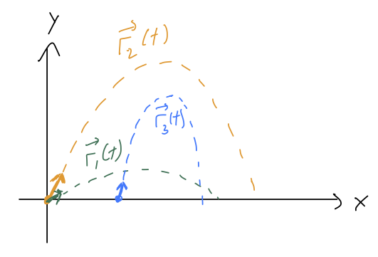
Now we know the 'next' values of position and velocity for our system. And since we know those, we plug in to the equation above and get the 'next' acceleration, \( d^2 \vec{r} / dt^2(\epsilon) \). Then we repeat the process to move to \( t = 2\epsilon \), and then \( 3\epsilon \), and so on until we've evolved as far as we want to in time. Depending on what choices we made for the initial values, we'll build up different curves for \( \vec{r}(t) \):
This might sound like a tedious procedure, and it is, but this process (or more sophisticated versions of it) are exactly how numerical solution of differential equations are found. If you use the "NDSolve" function in Mathematica, for instance, it's doing some version of this iterative procedure to give you the answer. But more importantly, I think this is a more physical way to think about what initial conditions mean, and why we need \( n \) of them for an \( n \)-th order ODE.
As a side benefit, this construction also established uniqueness of solutions, meaning that once we fully choose the initial conditions, there is only one possible answer for the solution to the ODE. For Newtonian physics, this means that knowing the initial position and velocity is enough to tell you the unique possible physical path \( \vec{r}(t) \) that the system will follow.
Linear ODEs and general solutions
Numerical solution is a great tool, but whenever possible we would prefer to be able to solve the equation by hand - this is more powerful because we can solve for a bunch of initial conditions at once, and we can have a better understanding of what the solution means.
To talk about analytic solutions, we have to introduce one more classification term, which is linear. To explain this clearly, remember that a linear function is one of the form
\[ \begin{aligned} y(x) = mx + b. \end{aligned} \]
To state this in words, the function only modifies \( x \) by addition and multiplication with some constants, \( m \) and \( b \). A linear differential equation, then, is one in which the unknown function and its derivatives are only multiplied by constants and added together.
For example, if we're solving for \( y(x) \), the most general linear differential equation looks like
\[ \begin{aligned} a_0(x) y + a_1(x) \frac{dy}{dx} + a_2(x) \frac{d^2y}{dx^2} + ... + b(x) = 0. \end{aligned} \]
This is a little more complicated since we have two variables now, but if you think of freezing the value of \( x \), then all of the \( a \)'s and \( b \) are constant and it's clearly a linear function.
A couple more examples, for clarity. These three ODEs are all linear:
\[ \begin{aligned} \frac{dy}{dx} + 3y = 1 \\ \frac{d^2u}{dt^2} + \sin^2 (t) u^2 = 0 \\ x^4 \frac{dy}{dx} + \frac{3x}{4x-5} y = e^x \end{aligned} \]
However, these two are non-linear:
\[ \begin{aligned} \frac{dy}{dx} + \frac{3}{y} = 1 \\ \frac{d^2u}{dt^2} = u^2 \end{aligned} \]
Linearity turns out to be a very useful condition. This isn't a math class so I won't go over the proof, but there is a very important result for linear ODEs:
_A linear ODE of order \( n \) has a unique general solution which depends on \( n \) independent unknown constants._
The term "general solution" means that there is a function we can write down which solves the ODE, no matter what the initial conditions are. This function has to contain \( n \) constants that can be adjusted to match initial conditions, but otherwise it is the same function everywhere.
(To avoid a common misconception, it's just as important to be aware of the opposite of this statement: if we have non-linear ODE, in many cases there is no general solution. There is still always a unique solution if we fully specify the initial values. But for a non-linear ODE the functional form of the solution can be different depending on what the initial values are! See Boas 8.2 for an example.)
Alright, so it's great that we know a general solution is out there, but how do we find it in practice? It's probably best to explain this using an example.
Example: a simple linear ODE
Let's solve the following ODE:
\[ \begin{aligned} \frac{d^2y}{dx^2} = +k^2 y \end{aligned} \]
There is a general procedure for solving second-order linear ODEs like this, but I'll defer that until later. To show off the power of general solutions, I'm going to use a much cruder approach: guessing. (If you want to sound more intellectual when you're guessing, the term used by physicists for an educated guess is "ansatz".)
Notice that the equation tells us that when we take the derivative of \( y(x) \) twice, we end up with a constant times \( y(x) \) again. This should immediately make you think about exponential functions, since \( d(e^x)/dx = e^x \). To get the constant \( k \) out from the derivatives, it should appear inside the exponential. So we can guess
\[ \begin{aligned} y_1(x) = e^{+kx} \end{aligned} \]
and easily verify that this indeed satisfies the differential equation. However, we don't have any arbitrary constants yet, so we can't properly match on to initial conditions. We can notice next that because \( y(x) \) appears on both sides of the ODE, we can multiply our guess by a constant and it will still work. So our refined guess is
\[ \begin{aligned} y_1(x) = Ae^{+kx}. \end{aligned} \]
This is progress, but we have only one unknown constant and we need two. Going back to the equation, we can notice that because the derivative occurs twice, a negative value of \( k \) would also satisfy the equation. So we can come up with a second guess:
\[ \begin{aligned} y_2(x) = Be^{-kx}. \end{aligned} \]
This is very similar to our first guess above, but it is in fact an independent solution, independent meaning that we can't just change the values of our arbitrary constants to get this form from the other solution. (We're not allowed to change \( k \), because it's not arbitrary, it's in the ODE that we're solving!)
Finally, we notice that the combination \( y_1(x) + y_2(x) \) of these two solutions is also a solution if we plug it back in. So we have
\[ \begin{aligned} y(x) = Ae^{+kx} + Be^{-kx} \end{aligned} \]
This is a general solution: it's a solution and it has two distinct unknown constants, \( A \) and \( B \). Thanks to the math result above, if we have a general solution to a linear ODE, we know that it is the general solution thanks to uniqueness.
The whole procedure we just followed might seem sort of arbitrary, and indeed it was, since it was based on guessing! For different classes of ODEs, there will be a variety of different solution methods that we can use. The power of the general solution for linear ODEs is that no matter how we get there, once we find a solution with the required number of arbitrary constants, we know that we're done. Often it's easiest to find individual functions that solve the equation, and then put them together as we did here.
Now let's start to look at some specific methods for solving differential equations. We're going to begin with first-order ODEs only, because that will open up a new class of physics problems for us to solve: projectile motion with air resistance. Later in the semester, we'll come back to second-order ODEs.
Separable first-order ODEs
A unique feature of first-order ODEs is that we can sometimes solve them just by doing integrals. A first-order ODE is separable if we can write it in the form
\[ \begin{aligned} F(y) dy = G(x) dx \end{aligned} \]
where \( F(y) \) and \( G(x) \) are just any arbitrary function. Once we've reached this form, we can just integrate both sides and end up with an equation relating \( y \) to \( x \), which is our solution.
A quick aside: splitting the differentials \( dy \) and \( dx \) apart like this is something physicists tend to do much more than mathematicians (although Boas does it!) Remember that \( dx \) and \( dy \) do have meaning on their own, as they're defined to be infinitesmal intervals when we define the derivative \( dy/dx \). That being said, if you're unsettled by the split derivative above, you can instead think of a separable ODE as one written in the form
\[ \begin{aligned} F(y) \frac{dy}{dx} = G(x) \end{aligned} \]
Then we can integrate both sides over \( dx \),
\[ \begin{aligned} \int F(y) \frac{dy}{dx} dx = \int G(x) dx \end{aligned} \]
The integral on the left becomes \( \int F(y) dy \) by a \( u \)-substitution. After we do the integrals, we just have a regular equation to solve for \( y \). The simplest case is when \( F(y) = 1 \), i.e. if we have
\[ \begin{aligned} \frac{dy}{dx} = G(x) \\ \int dy = \int G(x) dx \\ y = \int G(x) dx + C \end{aligned} \]
(notice that we get one overall constant of integration from the indefinite integrals, just as needed to match the single initial condition for a first-order ODE.)
Let's try a more interesting example.
Example: a separable first-order ODE
We'll solve the following ODE:
\[ \begin{aligned} x \frac{dy}{dx} - y = xy \end{aligned} \]
This might not be obviously separable, but let's do some algebra to find out. We'll put the \( y \)'s together first:
\[ \begin{aligned} x \frac{dy}{dx} = y(1+x) \end{aligned} \]
Then divide by \( x \) and by \( y \):
\[ \begin{aligned} \frac{1}{y} \frac{dy}{dx} = \frac{1+x}{x} \end{aligned} \]
Nice and separated! Next, we split the derivative apart and integrate on both sides:
\[ \begin{aligned} \int \frac{dy}{y} = \int dx\ \frac{1+x}{x} \end{aligned} \]
The left-hand side integral will give us the log of \( y \). On the right, it's easiest to just divide out and write it as \( 1/x + 1 \), which gives us two simple integrals:
\[ \begin{aligned} \ln y + C' = \int dx\ \left(1 + \frac{1}{x} \right) = x + \ln x + C'' \end{aligned} \]
Just to be explicit, I kept both unknown constants here since we did two indefinite integrals. But since \( C' \) and \( C'' \) are both arbitrary, and we're adding them together, we can just combine them into a single constant \( C = C'' - C' \).
Now we need to solve for \( y \). Start by exponentiating both sides:
\[ \begin{aligned} y(x) = \exp \left( x + \ln x + C'' \right) \\ = e^x e^{\ln x} e^{C''} \\ = B x e^x \end{aligned} \]
defining one more arbitrary constant. (Since we haven't determined what the constant is yet by applying boundary conditions, it's not so important to keep track of how we're redefining it.)
Finally, we can impose a boundary condition to find a particular solution. Let's say that \( y(2) = 2 \). We plug in to get an equation for \( B \):
\[ \begin{aligned} y(2) = 2 = 2B e^2 \\ \Rightarrow B = \frac{1}{e^2} = e^{-2} \end{aligned} \]
and so
\[ \begin{aligned} y(x) = xe^{x-2}. \end{aligned} \]
Exercise: a more physics-y separable ODE
Find the general solution:
\[ \begin{aligned} m \frac{dv}{dt} = -cv^2 \end{aligned} \]
with the initial condition \( v(0) = v_0 \).
(For those of you who have finished the reading already, you'll recognize this as the equation for quadratic air resistance.) As usual, try to give this a shot before you keep reading.
As implied, this is another separable ODE. In fact, since there is no explicit \( t \)-dependence at all, it's easy to separate out:
\[ \begin{aligned} \frac{dv}{v^2} = -\frac{c}{m} dt \end{aligned} \]
Now we integrate:
\[ \begin{aligned} -\frac{1}{v} = -\frac{c}{m} t + C' \end{aligned} \]
and invert:
\[ \begin{aligned} v(t) = \frac{1}{(c/m) t - C'} \end{aligned} \]
Now we have to apply the boundary condition. (You could also have done this before solving for \( v(t) \), the order doesn't matter.) Plugging in at \( t=0 \) gives a nice and simple relation,
\[ \begin{aligned} v(0) = v_0 = \frac{1}{-C'} \end{aligned} \]
or \( C' = -1/v_0 \). This gets rid of our last minus sign, and we find for the result
\[ \begin{aligned} v(t) = \frac{1}{(c/m)t + 1/v_0} = \frac{v_0}{1 + \frac{cv_0}{m} t}. \end{aligned} \]
We'll talk about the implications of this solution more once we've set up the physics context for air resistance properly.