Before we begin talking about air resistance, let's finish our discussion of ordinary differential equations with one more category and solution method.
Linear first-order ODEs
(Note: this solution is discussed in Boas 8.3, but I'm borrowing a little bit of terminology from later sections of chapter 8 to put it in context.)
Unfortunately, not all first-order ODEs are separable. However, it turns out that there is a nice and general way to attack linear first-order ODEs. The combination of linear and first-order is very restrictive: any such ODE must take the form
\[ \begin{aligned} \frac{dy}{dx} + P(x) y = Q(x). \end{aligned} \]
This is a good place to introduce one last technical term, which is homogeneous. A homogeneous ODE is one in which every single term depends on the unknown function \( y \) or its derivatives. The equation above does not satisfy this condition, because the \( Q(x) \) term on the right doesn't have any \( y \)-dependence; thus, we say this equation is inhomogeneous (some books will use "nonhomogeneous" instead.)
Now, there is another equation which closely related to the one above:
\[ \begin{aligned} \frac{dy_c}{dx} + P(x) y_c = 0. \end{aligned} \]
The "c" here stands for complementary; this equation is called the complementary equation to the original. Setting \( Q(x) \) to zero gives us an equation that is homogeneous. Better yet, this equation is separable too: we can readily find that
\[ \begin{aligned} \frac{dy_c}{y_c} = -P(x) dx \end{aligned} \]
or doing the integrals,
\[ \begin{aligned} y_c(x) = A e^{-\int dx P(x)}. \end{aligned} \]
Of course, this is only a solution if \( Q(x) \) happens to be zero. But it turns out to be part of the solution for any \( Q(x) \). Suppose that we are able to find some other function \( y_p(x) \), which is a particular solution that satisfies the original, inhomogenous equation. Then \( y(x) = y_c(x) + y_p(x) \) is also a solution of the full equation. This is easy to see by plugging in:
\[ \begin{aligned} \frac{dy}{dx} + P(x) y = \frac{d}{dx} \left( y_c(x) + y_p(x) \right) + P(x) (y_c(x) + y_p(x)) \\ = \left[\frac{dy_c}{dx} + P(x) y_c(x) \right] + \left[ \frac{dy_p}{dx} + P(x) y_p(x) \right] \\ = 0 + Q(x). \end{aligned} \]
This might not seem very useful, because we still have to find \( y_p(x) \) somehow. But notice that \( y_c(x) \) always has the arbitrary constant \( A \) in it. That means that \( y(x) = y_c(x) + y_p(x) \) is the general solution to our original ODE (the unique one, because it's linear, remember!)
Example: charging a capacitor
This isn't a mechanics example, but it happens to be one of the simpler cases of a first-order and inhomogeneous ODE problem, so let's do it anyway. We have an electric circuit consisting of a battery supplying voltage \( V_0 \), a resistor with resistance \( R \), and a capacitor with capacitance \( C \):
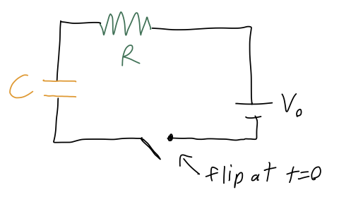
If the capacitor begins with no charge at \( t=0 \), we want to describe the current \( I(t) \) flowing in the circuit as a function of time. Now, current is the flow of charge, so the charge \( Q \) on the capacitor will satisfy the equation
\[ \begin{aligned} I = \frac{dQ}{dt}. \end{aligned} \]
The other relevant circuit equations we need are \( V = IR \) for the resistor, and \( Q = CV \) for the capacitor. Putting these together, we find that the equation describing the circuit is
\[ \begin{aligned} R \frac{dQ}{dt} + \frac{Q}{C} = V_0. \end{aligned} \]
The complementary equation is
\[ \begin{aligned} R\frac{dQ_c}{dt} + \frac{Q_c}{C} = 0 \end{aligned} \]
which is nice and separable:
\[ \begin{aligned} \frac{dQ_c}{Q_c} = -\frac{1}{RC} dt \end{aligned} \]
Integrating gives
\[ \begin{aligned} \ln Q_c = -\frac{t}{RC} + K \Rightarrow Q_c(t) = K' e^{-t/(RC)} \end{aligned} \]
Now we need to find the particular solution \( Q_p \). Fortunately, because the right-hand side is just a constant, it's easy to see that a constant value for \( Q_p \) will give us what we want. Specifically, if
\[ \begin{aligned} Q_p = CV_0 \end{aligned} \]
then the equation is satisfied, since the derivative term just vanishes.
Finally, we put things together and apply our boundary condition, \( Q(0) = 0 \):
\[ \begin{aligned} Q_c(0) + Q_p(0) = 0 = K' e^{-0/(RC)} + CV_0 = K' + CV_0 \end{aligned} \]
finding that \( K' = -CV_0 \), and thus the finished result is
\[ \begin{aligned} Q(t) = CV_0 \left(1 - e^{-t/(RC)} \right). \end{aligned} \]
So far, everything I've said is actually fairly general: this same approach with complementary and particular solutions will be something we use a lot when we get to second-order ODEs.
For any first-order linear ODE, there is actually a trick which will always give you the particular solution for any functions \( P(x) \) and \( Q(x) \). However, it's a little complicated to write down, and we won't need it often. So I won't cover that here, and instead I'll refer you to Boas 8.3 for the result. This is one of those formulas that you should know exists, but it's not worth memorizing - if you find you need it, you can go look it up.
Projectile motion and air resistance
Let's come back to physics and put our theory of first-order ODEs to use. Air resistance problems turn out to be the perfect application, because air resistance gives a force which depends on the velocity of the object moving through the air. Of course, Newton's second law is generally a second-order ODE,
\[ \begin{aligned} \vec{F} = m\ddot{\vec{r}}. \end{aligned} \]
But in the special case that the force only depends on the velocity \( \vec{v} = d\vec{r}/dt \), we can rewrite this as
\[ \begin{aligned} \vec{F}(\vec{v}) = m\dot{\vec{v}} \end{aligned} \]
which we can treat as a first-order ODE.
Before we get to the math, let's talk about the physics of air resistance, also known as drag for short (not to be confused with the regular friction that you get if you drag an object across a rough surface.) As the name implies, this is a force which resists motion, which explains why it depends on speed.
What do we know about the nature of the drag force \( \vec{f}(\vec{v}) \)? First of all, the air is (to a very good approximation) isotropic, i.e. it is uniform enough that it looks the same no matter which direction we move through it.
This means that the magnitude of the drag force should only depend on the speed, i.e. \( \vec{f}(\vec{v}) = \vec{f}(v) \). If the object moving through the air is also very symmetrical (like a sphere), then the orientation of our object also doesn't matter, and we expect the direction of the force to be opposite the direction of motion,
\[ \begin{aligned} \vec{f}(v) = -f(v) \hat{v}. \end{aligned} \]
There are many examples of systems for which this second equation does not hold. Taylor gives the example of an airplane, which experiences a lift force clearly not in the same direction of its motion. A more mundane example is a frisbee, for which air resistance actually provides a stabilizing force that keeps it from tumbling while in the air. But there are lots of interesting systems where this relation does hold, so we'll assume it for the rest of this section.
Unfortunately, this is still way too general: we need some information about what the function \( f(v) \) is before we can hope to make any progress. There are two effects that are important in the interactions between a fluid and an object traveling through it, and they will give us linear and quadratic dependence on the speed respectively. So the most general drag force we will study is
\[ \begin{aligned} f(v) = bv + cv^2. \end{aligned} \]
Now, Taylor points out that this is valid at "lower speeds", and that there are other effects that are important near the speed of sound. In fact, another way to derive this form for \( f(v) \) is through Taylor series expansion. But we should be careful, because this is a physics class, and series expanding in \( v \) doesn't really make sense - it has units! If we really want to expand, we need to expand in something dimensionless; equivalently, we need to answer the question "\( v \) is small compared to what?"
The answer is what I already said: \( v \) should be small compared to \( v_s \), the speed of sound of air (or whatever fluid medium we are studying.) \( v_s \) is the speed at which the motion of the air molecules relative to each other will start to matter and things will get more complicated. Thus, we can write
\[ \begin{aligned} f(v) = b_0\frac{v}{v_s} + c_0 \frac{v^2}{v_s^2} + d_0 \frac{v^3}{v_s^3} + ... \end{aligned} \]
(there is no constant term \( a_0 \), for the simple reason that we know there is no drag force if \( v=0 \).) The beauty of this approach is that so long as we are working at speeds \( v \ll v_s \), we can study air resistance even if we have no idea what the original function \( f(v) \) is: all we have to do is run a few experiments to measure the constants \( b_0, c_0, d_0 \) (and so on, if we care about even smaller corrections.)
This is another example of the concept of an effective theory: the series expansion version of \( f(v) \) is not valid at any speed, but at small speeds it can be used to make useful predictions once we've done a couple experiments to set it up. This should all remind you of the classical limit \( v \ll c \) from special relativity, too. I'll come back to the idea of effective theories again later on, but I want to point it out here because it's more common than you think.
Although the series-expansion theory approach would work just fine, we will instead borrow some more advanced ideas from fluid mechanics. There are two specific effects that will give rise to the linear and quadratic terms, and will thus allow us to predict what the coefficients \( b \) and \( c \) are.
Microscopic origin of drag forces
Let's begin with the linear drag force. From fluid mechanics, a constant known as the viscosity, \( \eta \), determines how resistant the air (or whatever fluid we are moving through) is to being deformed; larger \( \eta \) means that the force exerted by adjacent layers of fluid on each other is larger. Without going into too much detail, \( \eta \) has units of \( N \cdot s / m^2 \) (see Taylor problem 2.2.)
This is a low-speed effect which treats the air like a smooth, continuous medium. To see the dependence on the other properties of our moving object, consider this sketch:
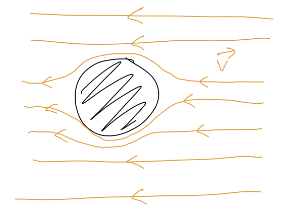
From the frame of reference of the moving object, the air is flowing across it at speed \( v \). Near the object itself, the moving air has its path deformed around the object; the size of the deformation is proportional to the linear size of the object, \( D \). The complete formula for a spherical object is
\[ \begin{aligned} f_{\rm lin}(v) = 3\pi \eta D v. \end{aligned} \]
where \( D \) is specifically the diameter of the sphere. For air at STP and a spherical object, Taylor goes on to give the result
\[ \begin{aligned} b = \beta D,\ \ \beta = 1.6 \times 10^{-4}\ N \cdot s / m^2 \end{aligned} \]
which is convenient for talking about air resistance in particular.
Next, we have the quadratic drag force. This is a more violent effect, arising at higher speeds. Basically, if the speed of our object is large enough, the air doesn't have enough time to flow smoothly out of the way, and instead the individual air molecules are swept up and kicked out of the path of our object:
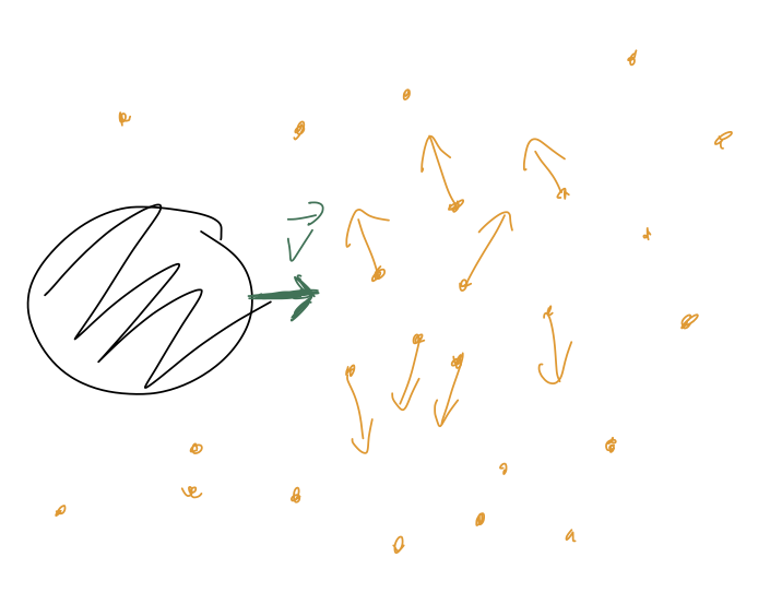
(This is an example of turbulent flow, as opposed to the smooth laminar flow in the linear regime.) We can think of there being two different \( v \)-dependent effects here. First, the speed at which the air molecules have to get out of the way will increase proportional to \( v \). Second, for larger \( v \) our object will simply run into more air molecules per unit time. So indeed, we expect a quadratic dependence \( v^2 \) for this force.
Two other factors influence how many air molecules are swept up per unit time. First, the cross-sectional area \( A \) of our object - the depth of the object doesn't matter because they're just scattering out of its path completely. Second, the density of the air, \( \rho \). (If we're counting molecules it's the number density \( \rho/m_{\rm air} \) that matters, but we're interested in the drag force, which puts the factor of \( m_{\rm air} \) back in.) Thus, the final result is
\[ \begin{aligned} f_{\rm quad}(v) = \frac{1}{2} C_D \rho A v^2 \end{aligned} \]
This introduces one more physical quantity, the dimensionless number \( C_D \) which is known as the drag coefficient. This number is usually between 0 and 1, and determines how streamlined the object is (for a smoother object, the air doesn't have to be deflected completely out of the way as soon as the front of the object hits it.) For a sphere, \( C_D \approx 0.5 \); a reasonably aerodynamic car has \( C_D \approx 0.25 \), and a 747 jumbo jet has \( C_D \approx 0.03 \).
Once again, we can specialize to air at STP and a spherical object, and Taylor gives the result
\[ \begin{aligned} c = \gamma D^2,\ \ \gamma = 0.25\ N \cdot s^2 / m^4. \end{aligned} \]
This is handy, but do keep in mind that it assumes a sphere; if you want to study air resistance for an object that you know the drag coefficient for, you should multiply by \( C_D / (1/2) = 2C_D \).
Next time, we'll talk about determining whether the linear or quadratic term (or neither) is dominant for a given problem, and then we'll move on to solving for the motion in the linear case.