Last time, we ended on discussing microscopic origins of the drag force, arriving (with some assumptions) at the form \( f(v) = bv + cv^2 \) for a force that always opposes the direction of motion, \( \vec{f}(\vec{v}) = -f(v) \hat{v} \).
Unfortunately, the general drag force \( f(v) = bv + cv^2 \) is still slightly too complicated to work with analytically for solving the motion. We will talk about that general case, but first we'll try to understand two restricted cases. In the linear drag regime, the \( bv \) term is relatively large and we can ignore the quadratic term completely; this is obviously where \( v \) is very small. In the other limit where \( v \) is very large, we can ignore the linear term and solve in the quadratic drag regime.
Of course, we can't just say "\( v \) is really big", we have to be quantitative - the size of \( b \) and \( c \) matters too! We should really just compare the forces directly:
\[ \begin{aligned} \frac{f_{\rm quad}}{f_{\rm lin}} = \frac{cv^2}{bv} = \frac{C_D \rho Av^2}{2 \eta D v} = \left( \frac{C_D A}{D^2} \right) \frac{D \rho v}{\eta} \end{aligned} \]
The combination \( C_D A / D^2 \) is some dimensionless number which is generally not very far from 1, while the other fraction is another dimensionless combination known as the Reynolds number,
\[ \begin{aligned} R \equiv \frac{D \rho v}{\eta}. \end{aligned} \]
So if \( R \ll 1 \), the linear force is definitely dominant and we can ignore the quadratic term. If \( R \gg 1 \), the opposite is true and we just study the quadratic term. If \( R \) is sort of close to 1, then we probably can't ignore either effect and need to be careful.
It's helpful to know the ratio of these forces for air and some example objects. In example 2.1, Taylor estimates that \( f_{\rm quad} / f_{\rm lin} \sim 600 \) for a baseball moving at 5 m/s, \( \sim 1 \) for a raindrop at 0.5 m/s, and \( \sim 10^{-7} \) at \( 5 \times 10^{-5} \) m/s in the Millikan oil drop experiment. From the way the Reynolds number depends on \( D \) and \( v \), this means that air resistance for everyday objects is almost always dominantly quadratic.
Following the book, let's start by solving the case of linear drag, which is less practically interesting but easier to work with mathematically.
Linear drag
The first example I will consider here is the simplest, which is horizontal motion with linear drag. (You can realize this experimentally by immersing a frictionless cart on a surface in some viscous liquid, like honey or molasses.) If we just start the cart off with some initial speed \( v_0 \) and release it, the only force acting will be drag:
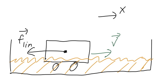
Newton's second law is thus
\[ \begin{aligned} m \ddot{x} = -b \dot{x}. \end{aligned} \]
As I said a little while back, we can turn this into a first-order ODE by taking \( v_x = \dot{x} \) as our unknown variable, leading to the equation
\[ \begin{aligned} \dot{v}_x = -\frac{b}{m} v_x. \end{aligned} \]
Better still, this is a separable ODE, so we can solve it right away. Separating \( v_x \) and \( t \) out gives
\[ \begin{aligned} \frac{dv_x}{v_x} = -\frac{b}{m} dt \end{aligned} \]
and then integrating leads to
\[ \begin{aligned} \ln v_x = -\frac{bt}{m} + C \Rightarrow v_x(t) = C' e^{-bt/m} \end{aligned} \]
and finally, using \( v_x(0) = v_0 \), the full solution is
\[ \begin{aligned} v_x(t) = v_0 e^{-t/\tau}, \end{aligned} \]
introducing the quantity \( \tau \equiv m/b \), sometimes called the "natural time" or "decay time". So, the speed as a function of time will decay to zero exponentially like so:
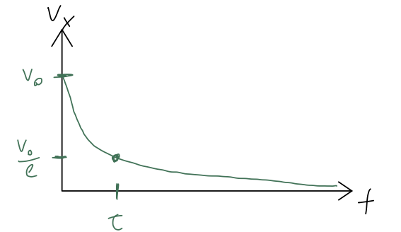
In fact, we could have guessed this qualitative behavior just from the equation of motion, before we solved it. Since the force is proportional to speed and acts to decrease the speed, the force is making itself smaller over time as the speed drops, with the "steady state" being reached at \( v_x = 0 \) where force is also zero.
Although we ignored the actual position \( x \) to get here, now that we have the solution, it's easy to reconstruct:
\[ \begin{aligned} x(t) = x(0) + \int_0^{t} dt' v_x(t') = x_0 + v_0 \int_0^t dt' e^{-t'/\tau} \\ = x_0 -\tau v_0 \left. e^{-t'/\tau} \right|_0^{t} \\ = x_0 + \tau v_0 (1 - e^{-t/\tau}). \end{aligned} \]
As \( t \) goes to infinity, the distance traveled by the cart approaches \( \Delta x_\infty = \tau v_0 \):
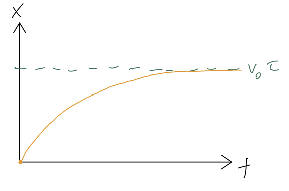
Notice that the natural time \( \tau \) popped up again: the total distance traveled by the cart when it stops is exactly the same as the distance it would have traveled with no drag in time \( \tau \). This isn't a deep statement: it's more of an example of dimensional analysis, which is the idea that we can often guess the right answer (or close to it) just by putting together known quantities in the only way that their units will allow. In this case, given \( v_0 \) and \( \tau \), the only thing we can build with units of distance is \( v_0 \tau \).
Now that we're warmed up, let's move on to the more interesting case of an object in freefall. We can restrict ourself to a single coordinate \( y \), and draw the free-body diagram:
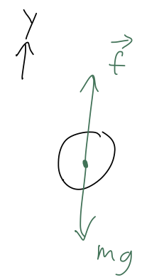
To avoid confusion, we need to be very careful about minus signs and what direction things are pointing in! Although I've drawn the free-body diagram assuming the velocity is pointing down, we can be general and say that \( \dot{y} \) can be either positive or negative. If you're comparing to Taylor, note that he assumes \( \vec{v} \) is pointing down and there are some minus-sign differences as a result.
The net force is
\[ \begin{aligned} \vec{F}_{\rm net} = -mg - f_{\rm lin}(\dot{y}) = -mg - b\dot{y} \end{aligned} \]
so the equation of motion is
\[ \begin{aligned} m\ddot{y} = -mg - b\dot{y}. \end{aligned} \]
and changing variables again to make it first order,
\[ \begin{aligned} \dot{v}_y = -g - \frac{b}{m} v_y. \end{aligned} \]
(Remember, \( v_y \) is positive for upwards motion, negative for downwards!) Before we move on to talk about solutions, we can already notice something interesting just from the equation of motion itself. There is a particular speed for which the right-hand side of the equation will vanish:
\[ \begin{aligned} v_{y} = -v_{\rm ter} = -\frac{mg}{b}. \end{aligned} \]
For an object free-falling at this speed, the drag force balances gravity and there is no acceleration. This speed is known as the terminal velocity, because it is the maximum possible speed that can be reached for an object dropped from rest. (Note that I took out a minus sign, so that the terminal velocity will always be a positive number, matching Taylor's definition.)
In fact, this is the final speed that will be reached for any initial speed, even if we launch an object faster than \( v_{\rm ter} \)! For \( vy < -v{\rm ter} \), the equation of motion tells us that \( \dot{v}y > 0 \), so the object will decelerate until it reaches \( v{\rm ter} \) and the forces balance.
Now let's find a solution. There is more than one way to do this: Taylor shows you one way involving a \( u \)-substitution. I'll use the fact that it's separable, instead. First, we should notice that this equation is inhomogeneous, because of the \( g \). The complementary equation is
\[ \begin{aligned} \dot{v}_{y,c} + \frac{b}{m} v_{y,c} = 0. \end{aligned} \]
We just solved this for horizontal motion; we know the answer is
\[ \begin{aligned} v_{y,c}(t) = Ce^{-bt/m}. \end{aligned} \]
Next, we need a particular solution. As before, because the inhomogeneous piece is just a constant, a constant particular solution will work: if we write
\[ \begin{aligned} v_{y,p}(t) = -\frac{mg}{b} = -v_{\rm ter}, \end{aligned} \]
then \( \dot{v}_{y,p} = 0 \) and the full equation is satisfied. Our general solution just requires putting them together:
\[ \begin{aligned} v_y(t) = v_{y,c}(t) + v_{y,p}(t) = -v_{\rm ter} + Ce^{-bt/m}. \end{aligned} \]
Finally, we apply our initial condition to fix the constant \( C \):
\[ \begin{aligned} v_y(0) = v_0 = -v_{\rm ter} + C \\ \Rightarrow C = v_0 + v_{\rm ter} \end{aligned} \]
or plugging back in, and putting in the natural time \( \tau = m/b \) like we did before,
\[ \begin{aligned} v_y(t) = v_0 e^{-t/\tau} - v_{\rm ter} (1 - e^{-t/\tau}). \end{aligned} \]
If \( v_0 = 0 \), this looks exactly like what the \( x \)-dependence looked like for the horizontal case: the speed starts at zero and grows like an inverse exponential, asymptoting towards the (negative) terminal velocity. More generally, the dependence on the initial speed \( v_0 \) will decay exponentially, so that as we discussed any solution will approach the terminal velocity at large enough times.
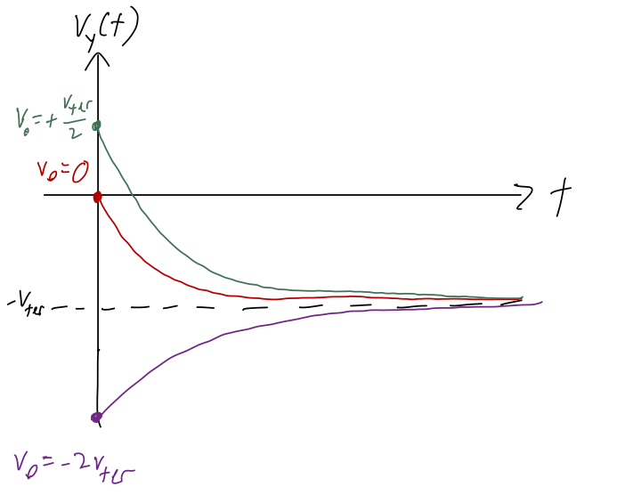
Exercise: sketching the solution for linear free-fall
Make a sketch of \( v_y(t) \) for two choices of initial conditions: \( v_y(0) = 0 \), and \( vy(0) = +v{\rm ter}/2 \).
A few general tips on sketching, here: always fill in important/known points and asymptotes first. Here we expect that all of our solutions asymptote at \( -v_{\rm ter} \), so that should be the first line you draw! Then I would fill in the y-intercepts, which are the initial conditions given to us.
From that point forward, you can finish the sketch, because you know it will be a smooth and exponentially decaying curve since all the time dependence is of the form \( e^{-t/\tau} \). (I wasn't careful about labelling \( t = \tau \) on my sketch below, but that would be a good addition, and would help you set the scale of your exponential curve!)
If you're having trouble visualizing the different pieces contributing here, try making a sketch or plot in Mathematica of the two terms separately, and then imagine the total curve as the sum of the two.
Here's a sketch with the two requested initial conditions, and another one beyond \( v_{\rm ter} \) just to show what happens in that case:
Finally, we can integrate once to get the position vs. time:
\[ \begin{aligned} y(t) = y(0) + \int_0^t dt' v_y(t') \\ = y_0 + v_0 \int_0^t dt' e^{-t'/\tau} - v_{\rm ter} \int_0^t dt' (1 - e^{-t'/\tau}) \\ = y_0 - \tau v_0 \left. e^{-t'/\tau} \right|_0^t - v_{\rm ter} t - \tau v_{\rm ter} \left. e^{-t'/\tau}\right|_0^t \\ = y_0 - v_{\rm ter} t + (v_0 + v_{\rm ter}) \tau (1 - e^{-t/\tau}). \end{aligned} \]
(Now we're back to agreeing exactly with Taylor (2.36), because he sneaks in a sign flip on \( v_{\rm ter} \) just above that equation.) Remember that \( v_{\rm ter} \) by definition is always positive, but we could have a negative \( v_0 \) if the initial velocity is pointing downwards.
Next time, we'll put our solutions together to look at projectile motion with linear drag. This will also lead us in to our next important math topic, which is power series.