I started this lecture by clarifying some statements from last time about handling air-resistance for non-spherical objects. Since the formulas \( b = \beta D \) and \( c = \gamma D^2 \) (as used in Taylor) assume a sphere moving through air at STP, we can use them as long as we're not looking for high precision and/or our object is close enough to spherical. For other cases, use the microscopic formulas - especially \( c = \frac{1}{2} C_D \rho A \) for quadratic drag, where the geometry of the object matters more than in the linear case.
Projectile motion with linear air resistance
Remember that one of the nice things about Newton's laws and Cartesian coordinates was that they just split apart into independent equations. In particular, suppose we want to study the problem of projectile motion in the \( x-y \) plane. The free-body diagram is:
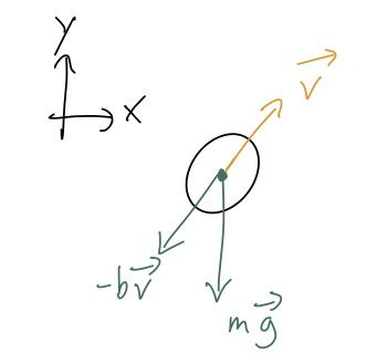
leading to the two equations of motion
\[ \begin{aligned} \ddot{x} = -\frac{b}{m} \dot{x}, \\ \ddot{y} = -g - \frac{b}{m} \dot{y}. \end{aligned} \]
Those are exactly the two equations we just finished solving for purely horizontal and purely vertical motion! So we can just take our solutions above and apply them. Separating out the individual components of initial speed, we have
\[ \begin{aligned} x(t) = x_0 + \tau v_{x,0} (1 - e^{-t/\tau}), \\ y(t) = y_0 - v_{\rm ter} t + (v_{y,0} + v_{\rm ter}) \tau (1 - e^{-t/\tau}). \end{aligned} \]
Usually when studying projectile motion, we are more interested in the path in \( (x,y) \) traced out by our flying object than we are in the time dependence. There is a neat trick to eliminate the time dependence completely, by noticing that the first equation is actually simple enough to solve for \( t \):
\[ \begin{aligned} \frac{x - x_0}{\tau v_{x,0}} = 1 - e^{-t/\tau} \\ \Rightarrow -\frac{t}{\tau} = \ln \left( 1 - \frac{x-x_0}{\tau v_{x,0}} \right) \end{aligned} \]
This is good enough to plug back in to the equation for \( y \):
\[ \begin{aligned} y - y_0 = v_{\rm ter} \tau \ln \left( 1 - \frac{x-x_0}{\tau v_{x,0}} \right) + (v_{y,0} + v_{\rm ter}) \tau \left( \frac{x-x_0}{\tau v_{x,0}}\right) \end{aligned} \]
or setting \( x_0 = y_0 = 0 \) for simplicity (it's easy to put them back at this point),
\[ \begin{aligned} y(x) = v_{\rm ter} \tau \ln \left( 1 - \frac{x}{\tau v_{x,0}} \right) + \frac{v_{y,0} + v_{\rm ter}}{v_{x,0}} x \end{aligned} \]
This is a little messy, and it also might be surprising: we know that in the absence of air resistance, projectiles trace out parabolas, so we should expect some piece of this to be proportional to \( x^2 \). But instead we found a linear term, and some complicated logarithmic piece.
We most definitely want to understand and compare this to the limit of removing air resistance - as always, considering limits is an important check! But it's not so simple to do here, because removing air resistance means taking \( b \rightarrow 0 \), but remember that the definition of the terminal velocity was \( v_{\rm ter} = mg/b \). The natural time \( \tau = m/b \) also contains the drag coefficient, so the limit we want is \( v_{\rm ter} \rightarrow \infty \) and \( \tau \rightarrow \infty \) at the same time!
To make sense of this result, and in particular to compare to the vacuum (no air resistance) limit, the best tool available turns out to be Taylor expansion. In fact, Taylor series are such a useful and commonly used tool in physics that it's worth a detour into the mathematics of Taylor series before we continue.
Power series and approximation of functions
All of the following discussion will be in the context of some unknown single-variable function \( f(x) \). Most of the formalism of series approximation carries over with little modification to multi-variable functions, but we'll focus on one variable to start for simplicity.
We begin by introducing the general concept of a power series, which is a function of \( x \) that can be written as an infinite sum over powers of \( x \) (hence the name):
\[ \begin{aligned} \sum_{n=0}^\infty a_n x^n = a_0 + a_1 x + a_2 x^2 + a_3 x^3 + ... \end{aligned} \]
Another way to state this definition is that a power series is an infinite-order polynomial in \( x \). The coefficients \( a_n \) are constants, but other than that for a general power series they can take on any values we want. Notice that the value \( x=0 \) is special: for any other \( x \) we need to know all of the \( a_n \) to calculate the sum, but at \( x=0 \) the sum is just equal to \( a_0 \). In fact, we can shift the location of this special value by writing the more general power series:
\[ \begin{aligned} \sum_{n=0}^\infty a_n (x-x_0)^n = a_0 + a_1 (x-x_0) + a_2 (x-x_0)^2 + a_3 (x-x_0)^3 + ... \end{aligned} \]
and now the sum is exactly \( a_0 \) at \( x=x_0 \). (Jargon: this second form is known as a power series about or around the value \( x_0 \).)
Now, if this was a math class we would likely talk about convergence, i.e. whether the result of this infinite sum can actually be calculated, which would depend on specifying some formula for what the \( a_n \) are. However, for our purposes I'm much more interested in the practical use of power series, and one of the most useful things we can do with a power series is to use it as an approximation to another function.
Suppose we have a "black box" function, \( f(x) \). This function is very complicated, so complicated that we can't actually write down a formula for it at all. However, for any particular choice of an input value \( x \), we can find the resulting numerical value of \( f(x) \). (In other words, we put the number \( x \) into the "box", and get \( f(x) \) out the other side, but we can't see what happened in the middle - hence the name "black box".)
Let's assume the black box is very expensive to use: maybe we have to run a computer for a week to get one number, or the numbers come from a difficult experiment. Then it would be very useful to have a cheaper way to get approximate values for \( f(x) \). To do so, we can define a power series by:
\[ \begin{aligned} f(x) = c_0 + c_1 x + ... + c_n x^n + ... \end{aligned} \]
(ignoring questions about convergence and domain/range, and just assuming this is possible.) The right-hand side is called a power-series representation of \( f(x) \). In principle, if we know a formula for all of the \( c_n \), then the sum on the right-hand side is the same thing as \( f(x) \). In practice, we can't use our black box infinity times. Instead, we can rely on a truncated power series, which means we stop at \( n \)-th order:
\[ \begin{aligned} f_n(x) \equiv c_0 + c_1 x + ... + c_n x^n. \end{aligned} \]
Now we just need to use the black box \( n+1 \) times with different values of \( x \), plug in to this equation, and solve for the \( c \)'s. We then have a polynomial function that represents \( f(x) \) that we can use to predict what the black box would give us if we try putting in a new value of \( x \).
This truncation is more or less required, but the most important question is: will the truncated function be a good approximation to the real \( f(x) \)? We can answer this by looking at the difference between the two, which I'll call the error, \( \delta_n \):
\[ \begin{aligned} \delta_n \equiv |f(x) - f_n(x)| = c_{n+1} x^{n+1} + ... \end{aligned} \]
So we immediately see the limitation: as \( x \) grows, \( \delta_n \) will become arbitrarily large. (Note that just the first term here lets us draw this conclusion, so we don't have to worry about the whole infinite sum.) The precise value of \( x \) where things break down depends on what the \( c \)'s are, and also on how much error we are willing to accept.
However, we can also make the opposite observation: as \( x \) approaches zero, this error becomes arbitrarily small! (OK, now I'm making some assumptions about convergence of all the higher terms. If the function \( f(0) \) blows up somehow, we'll be in trouble, but that just means we should expand around a different value of \( x \) where the function is nicer.) In the immediate vicinity of \( x=0 \), our power series representation will work very well. In other words, power-series representations are most accurate near the point of expansion.
As a quick example, here's what happens if I take \( f(x) = \cos(x) \), evaluate at three points, and find a truncated second-order power series representation. Using \( x=0,0.3,0.6 \) gives
\[ \begin{aligned} f_2(x) = 1 - 0.0066 x - 0.4741 x^2 \end{aligned} \]
Here's a plot comparing the power series to the real thing:
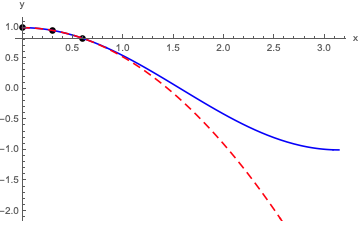
Obviously this works pretty well for \( x \leq 1 \) or so! For larger \( x \), it starts to diverge away from cosine. We can try to improve the expansion systematically if we add more and more terms before we truncate, although we have to worry about convergence at some point.
All of this is a perfectly reasonable procedure, but it's a little cumbersome since we have to plug in numerical values and solve. In the real world, of course, the numbers coming out of our "black box" probably also have uncertainties and we should be doing proper curve fitting, which is a topic for another class.
For our current purposes, what we really want is a way to find power-series representations when we know what \( f(x) \) is analytically, which brings us to the Taylor series.
Taylor series
(On notation: you may remember both the terms "Taylor series" and "Maclaurin series" as separate things. But the Maclaurin series is just a special case: it's a Taylor series about \( x=0 \). I won't use the separate term and will always just call this a Taylor series.)
Let's begin with a special case, and then I'll talk about the general idea of Taylor series expansion. Suppose we want a power-series representation for the function \( e^x \) about \( x=0 \):
\[ \begin{aligned} e^x = a_0 + a_1 x + a_2 x^2 + ... + a_n x^n + ... \end{aligned} \]
As we observed before, the value \( x=0 \) is special, because if we plug it in the series terminates - all the terms vanish except the first one, \( a_0 \). So we can easily find
\[ \begin{aligned} e^0 = 1 = a_0. \end{aligned} \]
No other value of \( x \) has this property, so it seems like we're stuck. However, we can find a new condition by taking a derivative of both sides:
\[ \begin{aligned} \frac{d}{dx} \left( e^x \right) = a_1 + 2 a_2 x + ... + n a_n x^{n-1} + ... \end{aligned} \]
So if we evaluate the derivative of \( e^x \) at \( x=0 \), now the second coefficient \( a_1 \) is singled out and we can determine it by plugging in! This example is especially nice, because \( d/dx(e^x) \) gives back \( e^x \), so:
\[ \begin{aligned} \left. \frac{d}{dx} \left( e^x \right) \right|_{x=0} = e^0 = 1 = a_1. \end{aligned} \]
We can keep going like this, taking more derivatives and picking off terms one by one:
\[ \begin{aligned} \frac{d^2}{dx^2} \left( e^x \right) = 2 a_2 + (3 \cdot 2) a_3 x + ... + n (n-1) a_n x^{n-2} + ... \\ \frac{d^3}{dx^3} \left( e^x \right) = (3 \cdot 2) a_3 + (4 \cdot 3 \cdot 2) a_4 x + ... + n (n-1) (n-2) a_n x^{n-2} + ... \end{aligned} \]
so \( a_2 = 1/2 \) and \( a_3 = 1/6 \). In fact, we can even find \( a_n \) this way: we'll need to take \( n \) derivatives to get rid of all of the \( x \)'s on that term, and the prefactor at that point will be
\[ \begin{aligned} n(n-1)(n-2)...(3)(2) = n! \end{aligned} \]
So the general formula is \( a_n = 1/n! \), and we can write out the power series in full as
\[ \begin{aligned} e^x = \sum_{n=0}^\infty \frac{x^n}{n!}. \end{aligned} \]
This is an example of a Taylor series expansion. A Taylor series is a power series which is obtained at a single point, by using information from the derivatives of the function we are expanding. As long as we can calculate those derivatives, this is a powerful method.
In the most general case, there are two complications that can happen when repeating what we did above for a different function. First, for most functions the derivatives aren't all 1, and their values will show up in the power series coefficients. Second, we can expand around points other than \( x=0 \). The general form of the expansion is:
\[ \begin{aligned} f(x) = \sum_{n=0}^\infty f^{(n)}(x_0) \frac{(x-x_0)^n}{n!} \\ = f(x_0) + f'(x_0) (x-x_0) + \frac{1}{2} f''(x_0) (x-x_0)^2 + \frac{1}{6} f'''(x_0) (x-x_0)^3 + ... \end{aligned} \]
where here I'm using the prime notation \( f'(x) = df/dx \), and \( f^{(n)}(x) = dnf/dxn \) to write the infinite sum.
For most practical uses, the infinite-sum version of this formula isn't the most useful: functions like \( e^x \) where we can calculate a general formula for all of the derivatives to arbitrarily high order are special cases. Instead, we will usually truncate this series as well. The Taylor series truncated at the \( (x-x_0)^n \) is called the \( n \)-th order series; by far the most commonly used are first order (a.k.a. linear) and second order (a.k.a. quadratic.) The names follow from the fact that these series approximate \( f(x) \) as either a linear or quadratic function in the vicinity of \( x_0 \):
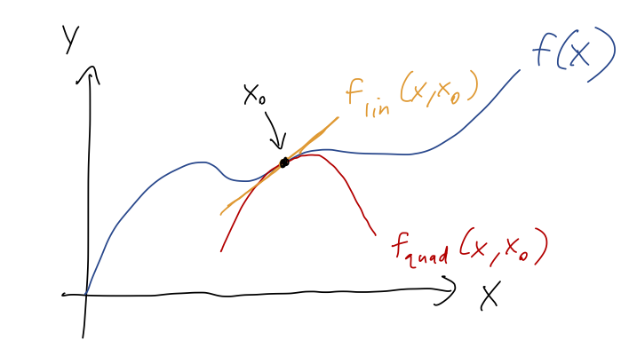
where the extra curves I drew are just the truncated Taylor series,
\[ \begin{aligned} f_{\rm lin}(x,x_0) = f(x_0) + f'(x_0) (x-x_0) \\ f_{\rm quad}(x,x_0) = f(x_0) + f'(x_0) (x-x_0) + \frac{1}{2} f''(x_0) (x-x_0)^2 \\ \end{aligned} \]
Even though we usually only need a couple of terms, one of the nice things about Taylor series is that for analytic (i.e. smooth and well-behaved) functions, which are generally what we encounter in physics, the series will always converge. So if we need to make systematic improvements to our approximation, all we have to do is calculate more terms.
Example: a simple Taylor series
Let's do a simple example: we'll find the Taylor series expansion of
\[ \begin{aligned} f(x) = \sin^2(x) \end{aligned} \]
up to second order. We start by calculating derivatives:
\[ \begin{aligned} f'(x) = 2 \cos (x) \sin(x) \\ f''(x) = -2 \sin^2 (x) + 2 \cos^2(x) \end{aligned} \]
This gives us enough to find the Taylor series to quadratic order about any point we want. For example, if we expand at \( x=0 \), then \( \sin(0) = 0 \) and \( \cos(0) = 1 \) gives
\[ \begin{aligned} f'(0) = 0 \\ f''(0) = 2 \end{aligned} \]
and thus
\[ \begin{aligned} \sin^2(x) \approx 0 + 0 x + \frac{1}{2!} (2) x^2 + ... = x^2 + \mathcal{O}(x^3). \end{aligned} \]
This introduces the big-O notation, which denotes order: it says that all of the missing terms are at least of order \( x^3 \), i.e. they're proportional to \( x^3 \) or even higher powers.
We'll come back and finish the example next time!