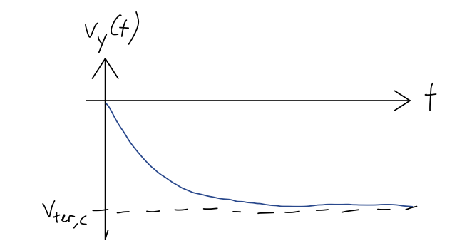
Last time, we ended on the following solution for freefall with quadratic drag when the initial speed is zero:
\[ \begin{aligned} v_y(t) = v_{{\rm ter},c} \frac{e^{-2t/\tau} - 1}{e^{-2t/\tau} + 1}. \end{aligned} \]
First, notice that the exponential pieces are always less than 1, so the fraction is always negative, which it had better be because we assumed \( v_y < 0 \)! As \( t \rightarrow \infty \), the exponentials vanish, and we approach the terminal velocity asymptotically, like in the linear case.
What about the hyperbolic trig function? Let's review those very quickly. The definitions of hyperbolic sine and cosine are
\[ \begin{aligned} \sinh(x) = \frac{1}{2} (e^x - e^{-x}) \\ \cosh(x) = \frac{1}{2} (e^x + e^{-x}) \end{aligned} \]
At large negative and positive \( x \), these are dominated by one or the other exponential. So the whole functions resemble two exponential curves stuck together, with or without a minus sign:
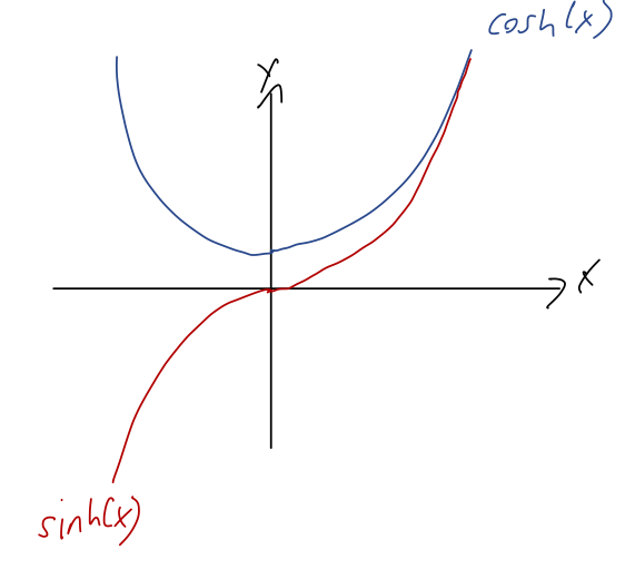
The reason these are called hyperbolic trig functions is that they satisfy a number of identities that are similar to the regular trig identities: for example, \( \cosh^2 x - \sinh^2 x = 1 \). (Aside: the real reason is because you can define them by trying to do trigonometry using a unit hyperbola instead of a unit circle, and the deeper reason is that they're actually related to ordinary trig functions once you start using complex numbers.)
Finally, the hyperbolic tangent is defined in analogy to the regular tangent:
\[ \begin{aligned} \tanh(x) = \frac{\sinh(x)}{\cosh(x)} =\frac{e^x - e^{-x}}{e^x + e^{-x}} = \frac{e^{2x} - 1}{e^{2x} + 1}. \end{aligned} \]
Here's a sketch of that function, showing the asymptotes at \( \pm 1 \):
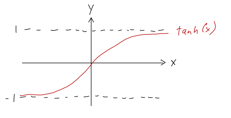
This function comes up frequently in physics - we've just seen an example - but the fact that it smoothly goes from \( -1 \) to \( +1 \) makes it useful in a variety of engineering applications as well, because it maps an arbitrary input signal into a finite range. One example is in machine learning, where the response of individual neurons in a neural net is often modeled with \( \tanh \).
Thus, for the special case of starting at rest, we can write our solution simply as a hyperbolic tangent:
\[ \begin{aligned} v_y(t) = -v_{{\rm ter},c} \tanh \left( \frac{t}{\tau} \right) = -v_{{\rm ter},c} \tanh \left( \frac{gt}{v_{{\rm ter},c}} \right). \end{aligned} \]
This is nice and simple, but it's also only true if we start at rest! For \( v_0 \neq 0 \), the general solution is
\[ \begin{aligned} v_y(t) = v_{{\rm ter},c} \frac{(v_{{\rm ter},c} + v_0) e^{-2t/\tau} - (v_{{\rm ter},c} - v_0)}{(v_{{\rm ter},c} + v_0) e^{-2t/\tau} + (v_{{\rm ter},c} - v_0)} \end{aligned} \]
which can't be written as a hyperbolic tangent in any particularly nice way. (This is a good reminder that it's important to carry your integration constants along when solving ODEs! If you just solved at rest, you might be tempted to think that the general solution for a moving initial condition would just be to add \( v_0 \) to the \( \tanh(...) \) solution above - but that would be wrong!)
One final thing to point out, linking back to our general discussion of ODEs. Remember that this is a non-linear ODE, for which we were warned that we can't necessarily find a general solution. What we just found looks general, but don't forget that we had to assume \( v_y < 0 \). If instead we had taken \( v_y > 0 \), a very important minus sign would be flipped, and the key integral above would become
\[ \begin{aligned} \int \frac{du}{1+u^2} = \tan^{-1}(u). \end{aligned} \]
So solutions for positive initial speed look like regular tangent instead of hyperbolic tangent. In other words, the functional form of our solution changes depending on initial conditions! This is always a possibility if our ODE is non-linear.
Example: oops!
I accidentally drop my wedding ring (mass ~ 10 g, width ~ 6 mm) into a glass of dark beer. Beer is more viscous than air, by a factor of about 137 according to Wikipedia; it's also more dense than air, by a factor of about 750.
a) Is linear or quadratic drag dominant? b) What is the terminal velocity? c) How long will it take to hit the bottom of a 15-cm tall pint glass, using a first-order series expansion? Is this result trustworthy?
Starting with part a), I know how the drag coefficients scale with viscosity and density,
\[ \begin{aligned} \beta = 3\pi \eta,\ \ \gamma = \frac{1}{2} C_D \rho (A/D^2). \end{aligned} \]
The important part is that \( \beta \) is linear in the viscosity \( \eta \), and \( \gamma \) is linear in medium density \( \rho \). Comparing to air as a baseline, the density goes up more than the viscosity does, so \( \gamma \) will increase more than \( \beta \). Because we know that everyday objects tend to be quadratic-drag dominated in air, this will probably still be true in the beer, so this should be a quadratic drag problem.
Just to be thorough, I'll calculate both drag coefficients, using Taylor's values for air and \( D = 6 \) mm:
\[ \begin{aligned} b = \beta_{\rm air} \frac{\eta_{\rm beer}}{\eta_{\rm air}} D \\ = (1.6 \times 10^{-4}\ {\rm N} \cdot {\rm s} / {\rm m}^2) (137) (6\times 10^{-3}\ {\rm m}) \\ = 1.3 \times 10^{-4}\ {\rm N} \cdot {\rm s} / {\rm m} \end{aligned} \]
and
\[ \begin{aligned} c = \gamma_{\rm air} \frac{\rho_{\rm beer}}{\rho_{\rm air}} D^2 \\ = (0.25\ {\rm N} \cdot {\rm s}^2 / {\rm m}^4) (750) (6 \times 10^{-3}\ {\rm m})^2 \\ = 6.8 \times 10^{-3}\ {\rm N} \cdot {\rm s}^2 / {\rm m}^2. \end{aligned} \]
So the Reynolds number is
\[ \begin{aligned} R = \frac{cv}{b} = \frac{v}{0.019\ {\rm m}/{\rm s}}. \end{aligned} \]
As long as the terminal velocity for quadratic drag isn't too close to \( 0.019\ {\rm m}/{\rm s} \), then, we expect the quadratic force to dominate.
On to part b), which is simple: we just plug in to the formula for quadratic freefall and find
\[ \begin{aligned} v_{\rm ter,c} = \sqrt{\frac{mg}{c}} = \sqrt{\frac{(10^{-2}\ {\rm kg})(9.8\ {\rm m}/{\rm s}^2)}{6.8 \times 10^{-3}\ {\rm N} \cdot {\rm s}^2 / {\rm m}^2}} \approx 3.8\ {\rm m}/{\rm s}. \end{aligned} \]
This is safely large enough that our Reynolds number will be very large for the majority of the motion, so the quadratic model is okay. For good measure, we should also calculate the natural time:
\[ \begin{aligned} \tau = \frac{g}{v_{\rm ter,c}} = 2.6\ {\rm s}. \end{aligned} \]
Finally, we ask about series expansion of the answer - although we know the full solution in this case, it's still useful to think about to improve our understanding of series expansion use in general. As we just found, the full solution starting from rest is
\[ \begin{aligned} v_y(t) = -v_{\rm ter,c} \tanh \left( \frac{t}{\tau} \right) \end{aligned} \]
We could look up a formula for the series expansion of \( \tanh \), or look up its derivatives and expand ourselves, but I'll use a trick to find the expansion to first order instead. Recall the definition:
\[ \begin{aligned} \tanh(x) = \frac{e^{2x} - 1}{e^{2x} + 1} \end{aligned} \]
Now I'll apply the series expansions for \( e^{2x} \):
\[ \begin{aligned} \tanh(x) = \frac{1 + 2x + 2x^2 + ... - 1}{1 + 2x + 2x^2 + ... + 1} = \frac{x+...}{1+x+...} \end{aligned} \]
cancelling off a 2. We're still not finished, since this isn't a polynomial yet. But we can use the expansion \( 1/(1+x) = 1-x + ... \) to move the denominator up top,
\[ \begin{aligned} \tanh(x) = (x+...) (1 - x + ...) = x + \mathcal{O}(x^2) \end{aligned} \]
Actually, there is no \( \mathcal{O}(x^2) \) term at all, because of the relation \( \tanh(-x) = -\tanh(x) \). So the missing terms start at \( \mathcal{O}(x^3) \). From this expansion, we have
\[ \begin{aligned} v_y(t) \approx -v_{\rm ter,c} \frac{t}{\tau} \end{aligned} \]
and then
\[ \begin{aligned} y(t) \approx \int_0^t\ v_y(t')\ dt' = -\frac{v_{\rm ter,c} t^2}{2\tau} \\ \Rightarrow t = \sqrt{\frac{2h\tau}{v_{\rm ter,c}}} \end{aligned} \]
where \( h \) is the drop height. Plugging in numbers gives \( t \approx 0.45 \) s.
Now, the final question: do I trust the series expansion result? This is a question about error due to series expansion, usually we would state the condition to use the expansion as "\( t \ll \tau \)". But let's be more precise. By using a series expansion, the error we're making is roughly the size of the first missing term in the expansion, which is proportional to \( (t/\tau)^3 \). If we had kept that term, our formula for \( v_y(t) \) would have been
\[ \begin{aligned} v_y(t) \approx -v_{\rm ter,c} \frac{t}{\tau} \left(1 + K \frac{t^2}{\tau^2} \right), \end{aligned} \]
where to figure out \( K \) we'd have to compute the Taylor expansion out to third order. If we really want to be careful, we can do just that, but instead let's assume \( K \) is not too far from 1. Then what matters is the size of \( t2/\tau2 \), which is
\[ \begin{aligned} \frac{t^2}{\tau^2} \approx 0.03. \end{aligned} \]
So, up to the size of whatever the number \( K \) turns out to be, we're making an error of around 3% in \( v_y(t) \) by using the first-order series expansion. The first observation we can make is that since this is much smaller than 1, we don't have to worry about convergence of the series, i.e. the first-order answer is a good initial guess.
Beyond that, do we need to go find the next term in the expansion? If I'm just observing this process happening by eye, then probably not; I don't think a human observer would easily notice differences on the order of a few hundredths of a second. On the other hand, if I want to know the answer to within 1% accuracy - maybe if I want to make measurements of this kind of motion to work backwards and calculate the density of the beer, for example - then I do need to keep the next term in the series.
To summarize: the order at which we stop is always found by the accuracy at which we need the answer; and (as long as the series converges!) we can always get better accuracy by continuing the expansion to the next order.