Projectiles with quadratic resistance; linear + quadratic resistance
At this point, the obvious next step would be to try to put our solutions together to study projectile motion with quadratic drag. Unfortunately, there's an obstacle to doing this that wasn't present in the linear case, which we can see if we go back to the vector form of Newton's second law. In the linear case, we have
\[ \begin{aligned} \vec{F} = m\dot{\vec{v}} = m\vec{g} - bv \hat{v} = m\vec{g} - b\vec{v}. \end{aligned} \]
This splits cleanly into two separate equations for \( v_x \) and \( v_y \), because only \( \vec{v} \) appears on both sides. However, in the quadratic case, the general equation is
\[ \begin{aligned} m\dot{\vec{v}} = m\vec{g} - cv^2 \hat{v} = m\vec{g} - cv \vec{v}. \end{aligned} \]
This almost splits up in the same way, but we have an extra factor of \( v \), which is the overall speed. If we write this full equation out in components, we find
\[ \begin{aligned} \dot{v}_x = -\frac{c}{m} \sqrt{v_x^2 + v_y^2} v_x \\ \dot{v}_y = -g - \frac{c}{m} \sqrt{v_x^2 + v_y^2} v_y. \end{aligned} \]
These are non-linear ODEs, but even worse they're coupled ODEs, meaning that we have to solve them simultaneously because each equation depends on the other unknown velocity component. In fact, the only way we can deal with these more complicated equations is to solve them numerically. Taylor talks a little bit about this, but I'll let you read his example and will not say any more here.
We run into a similar problem if we try to solve the general case of having both linear and quadratic drag forces,
\[ \begin{aligned} m\dot{\vec{v}} = m\vec{g} - b\vec{v} - cv \vec{v} \end{aligned} \]
which would be required when the Reynolds number is close to 1. It is actually possible to solve the horizontal- and vertical-motion cases analytically here, but those full solutions won't show off anything new and interesting in terms of either physics or math, so we'll skip over them. The full study of projectile motion with both terms can only be done numerically due to the quadratic term.
Momentum and conservation laws
Our next big physics topic is going to be momentum, both the ordinary kind and the rotational kind (i.e. angular momentum.) Although we've sort of been ignoring it when solving problems, the concept of momentum is central to all three of Newton's laws, and in fact the way we write the second law,
\[ \begin{aligned} \vec{F} = m \ddot{\vec{r}}, \end{aligned} \]
is actually not always correct! The most general correct form of Newton's second law is actually the one stated in terms of momentum,
\[ \begin{aligned} \vec{F} = \dot{\vec{p}}. \end{aligned} \]
This is the version that applies when we extend mechanics to include special relativity. It's also the version that applies in the case that \( m \) depends on time - the most important example of such a system is a rocket, which we'll be studying in detail.
Momentum is also a really useful concept because it obeys a conservation law, which you've certainly learned in intro physics and which we'll re-derive next. The general idea of a conservation law is simple: if \( C \) is some property of a physical system, then we say that \( C \) is conserved if
\[ \begin{aligned} \frac{dC}{dt} = 0, \end{aligned} \]
i.e. if \( C \) doesn't change with time. This is a simple but really powerful observation! Having a conservation law lets us do several useful things:
- If we know the starting and ending points of our system, we can calculate \( C_{\rm initial} \) and \( C_{\rm final} \), and they must be equal.
- If there are parts within \( C \) that do depend on time, then setting \( dC/dt = 0 \) can give us a useful and relatively simple differential equation relating them.
- A conservation law can give us powerful qualitative insights about how different parts of a physical system interact with each other and with the outside world. For example, energy conservation means that there is no such thing as "free energy" - if a black box is producing mechanical energy, it has to be transferred from somewhere!
There is an even deeper connection between conservation laws and symmetries, which are ways in which you can change an experiment without changing the result. Probably the most important symmetry in nature, and the reason that science can work at all, is known as time translation symmetry: the fact that if you wait a little while after an experiment and then repeat it (being careful to reset the initial conditions), the outcome will be the same. It turns out that this all-important symmetry actually leads to one of the most important conservation laws, conservation of energy. Unfortunately, the framework to prove that is something you won't see until next semester, so you'll have to stick around to see it!
Conservation of linear momentum
Now let's dig into the first important conservation law we'll discuss, conservation of linear momentum. I'll state it first:
"For any physical system which is subject to zero net external force, the total combined linear momentum \( \vec{P} \) of all objects in that system satisfies \( d\vec{P}/dt = 0 \)."
This can be thought of an extension of Newton's second law, since \( \vec{F} = \dot{\vec{p}} \) immediately tells us that for a single point mass, its momentum is conserved with no force acting on it. The more subtle point is that we're claiming this is true even for a system of masses. So the second-law approach will only work if we can also show that \( \vec{F}_{\rm ext} \), the net external force, is equal to \( \dot{\vec{P}} \), the rate of change of total momentum.
To work this out in general, we'll say that we have a collection of \( N \) point masses, with masses \( m_1, m_2, ..., m_N \). They can all move independently, so we'll also have to keep track of \( N \) momentum vectors \( \vec{p}_1, \vec{p}_2, ..., \vec{p}_N \). (Likewise there are \( N \) position vectors \( \vec{r}_1, ..., \vec{r}_N \), but we won't need to refer to them for present purposes.)
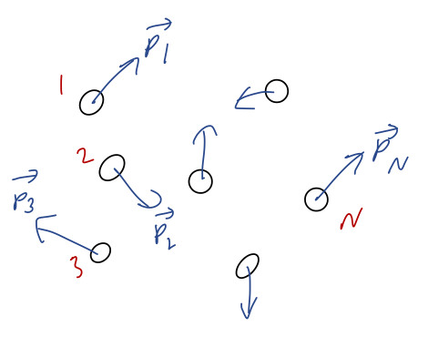
Let's start by just focusing on the first two masses, 1 and 2. To be completely general, there can be forces acting between these two particles in either direction. (Our collection could be a liquid, or a solid, in which case we have bonding forces; it could be a bunch of asteroids, which would have a gravitational force; it could be a collection of electric charges.) We can divide up the net force on each object to single out that piece:
\[ \begin{aligned} \vec{F}_1 = \vec{F}_{12} + \vec{F}_{1,\rm{ext}} \\ \vec{F}_2 = \vec{F}_{21} + \vec{F}_{2,\rm{ext}} \end{aligned} \]
where \( \vec{F}1 \) is the net force acting on mass 1, \( \vec{F}{12} \) can be read as "the force on mass 1 by mass 2", and \( \vec{F}_{1,\rm{ext}} \) just represents all other forces external to the mass 1 - mass 2 system.
Now, we know that Newton's second law will hold for each of our two masses, so
\[ \begin{aligned} \vec{F}_1 = \frac{d\vec{p}_1}{dt},\ \ \vec{F}_2 = \frac{d\vec{p}_2}{dt}. \end{aligned} \]
This means that if we define the total momentum \( \vec{P_{12}} \equiv \vec{p}_1 + \vec{p}_2 \), then
\[ \begin{aligned} \frac{d\vec{P}_{12}}{dt} = \vec{F}_1 + \vec{F}_2 = \vec{F}_{1,\rm{outside}} + \vec{F}_{2,\rm{ext}} + \vec{F}_{12} + \vec{F}_{21}. \end{aligned} \]
But now, we can call on Newton's third law: the net forces between objects 1 and 2 must be equal and opposite, \( \vec{F}{21} = -\vec{F}{12} \). This means that the last two terms above cancel, and we just have
\[ \begin{aligned} \frac{d\vec{P}_{12}}{dt} = \sum_{\alpha=1}^2 \vec{F}_{\alpha,\rm{ext}} = \vec{F}_{\rm net, ext}. \end{aligned} \]
(On the last line I used summation notation to rewrite the sum of two outside forces, and then combined them into a single net force. We'll be using sums a lot when we move past two masses!) So for two masses in isolation, we find that the combination of Newton's second and third laws allows us to conclude that the combined momentum satisfies Newton's second law, in terms of the outside forces acting on the pair; the momentum change due to the internal forces cancelled out in the sum.
Seeing that it works in the simple case, let's move on to the full set of \( N \) particles. The manipulations we need to do will be similar, but we'll have to keep track of all of the pieces. Let's start with mass 1 again, singling out the force on it due to each other particle:
\[ \begin{aligned} \vec{F}_1 = \vec{F}_{12} + \vec{F}_{13} + ... + \vec{F}_{1N} + \vec{F}_{1,\rm{ext}} \\ = \sum_{\alpha=2}^N \vec{F}_{1\alpha} + \vec{F}_{1,\rm{ext}} \end{aligned} \]
using summation notation to write this more compactly. Similarly for the second mass,
\[ \begin{aligned} \vec{F}_2 = \vec{F}_{21} + \vec{F}_{23} + ... + \vec{F}_{2N} + \vec{F}_{2,\rm{ext}} \\ = \sum_{\alpha \neq 2} \vec{F}_{2\alpha} + \vec{F}_{2,\rm{ext}} \end{aligned} \]
where we're adopting a new notation for the sum, which means "sum over all possible values of \( \alpha \), except for \( \alpha = 2 \)" - which is missing because mass 2 can't exert any force on itself. (In this notation it's implied that \( \alpha \) runs from 1 to \( N \), instead of explicitly written on the symbol.) Seeing the pattern, we can write for an arbitrary mass \( \beta \)
\[ \begin{aligned} \vec{F}_\beta = \sum_{\alpha \neq \beta} \vec{F}_{\beta \alpha} + \vec{F}_{\beta, \rm{ext}}. \end{aligned} \]
Newton's second law tells us that \( \vec{F}\beta = d\vec{p}\beta/dt \). As before, our next step is to put together the total momentum of the system,
\[ \begin{aligned} \vec{P} = \sum_\beta \vec{p}_\beta. \end{aligned} \]
Now we take the time derivative and apply Newton's second law:
\[ \begin{aligned} \frac{d\vec{P}}{dt} = \sum_\beta \frac{d\vec{p}_\beta}{dt} = \sum_\beta \vec{F}_\beta \\ = \sum_\beta \left( \sum_{\alpha \neq \beta} \vec{F}_{\beta \alpha} + \vec{F}_{\beta, \rm{ext}} \right). \end{aligned} \]
Let's focus on the first "sum of sums", the sum over all internal forces; in line with our 2-mass example, we expect this to add up to zero due to Newton's third law. To see any cancellation happening, we'll have to split this apart into pieces somehow. We can accomplish that by splitting apart the \( \neq \) sign:
\[ \begin{aligned} \sum_\beta \sum_{\alpha \neq \beta} \vec{F}_{\beta \alpha} = \sum_\beta \sum_{\alpha < \beta} \vec{F}_{\beta \alpha} + \sum_\beta \sum_{\alpha > \beta} \vec{F}_{\beta \alpha} \end{aligned} \]
Now, we do the following trick on the second sum: since the labels \( \alpha \) and \( \beta \) are arbitrary (like variables of integration), we can swap them. Then we notice that because the double sum means "sum over all pairs \( (\alpha, \beta) \) where \( \beta > \alpha \)", we can invert the order of the sums and rewrite the inequality:
\[ \begin{aligned} \sum_\beta \sum_{\alpha > \beta} \vec{F}_{\beta \alpha} = \sum_\alpha \sum_{\beta > \alpha} \vec{F}_{\alpha \beta} = \sum_{\beta} \sum_{\alpha < \beta} \vec{F}_{\alpha \beta} \end{aligned} \]
Putting things back together gives
\[ \begin{aligned} \sum_\beta \sum_{\alpha \neq \beta} \vec{F}_{\beta \alpha} = \sum_\beta \sum_{\alpha < \beta} (\vec{F}_{\beta \alpha} + \vec{F}_{\alpha \beta}) \end{aligned} \]
and finally using the third law, \( \vec{F}{\alpha \beta} = -\vec{F}{\beta \alpha} \), so this sum just vanishes! Thus, we have the result we wanted,
\[ \begin{aligned} \frac{d\vec{P}}{dt} = \vec{F}_{\rm{net, ext}}. \end{aligned} \]
Part of the reason we're doing this exercise with sums is so that you can get a little bit of experience in this kind of sum manipulation where we switch indices around. In case those index-manipulation steps went too fast for you, and in general for sum problems like this, it can be a good idea to write things out more explicitly. Here's what the terms in the sum look like without summation notation, excluding the \( \vec{F}_{\rm ext} \) pieces:
\[ \begin{aligned} \vec{F}_{1,{\rm int}} = 0 + \vec{F}_{12} + \vec{F}_{13} + ... + \vec{F}_{1N} \\ \vec{F}_{2,{\rm int}} = \vec{F}_{21} + 0 + \vec{F}_{23} + ... + \vec{F}_{2N} \\ \vec{F}_{3,{\rm int}} = \vec{F}_{31} + \vec{F}_{32} + 0 + ... + \vec{F}_{3N} \\ ... \end{aligned} \]
I've explicitly written zeroes in place of the ''missing'' diagonal terms \( \vec{F}{11}, \vec{F}{22}... \) to make the pattern more obvious. For the few terms we've written out, we see the third-law cancellation: every \( \vec{F}{\alpha \beta} \) has a corresponding \( \vec{F}{\beta \alpha} \) on the opposite side of the diagonal.
We can also now see what the arcane sum manipulations I did above mean more explicitly. When we divide up the sum over \( \alpha \neq \beta \), the \( \alpha < \beta \) piece of \( \vec{F}_{\beta \alpha} \) is all the terms below the diagonal, while \( \alpha > \beta \) is the terms above. But saying "all possible \( \vec{F}_{\alpha \beta} \) where \( \alpha < \beta \)" is clearly also all the terms above the diagonal.
So we've shown that the total momentum of any collection of physical objects changes only according to the net external force. This is a very powerful result! In particular, momentum conservation will let us make detailed statements about mechanics problems without knowing anything about the (often very complicated!) internal forces at work. Here are a few nice examples, briefly:
- Inelastic collisions: for example, a car crash certainly involves a lot of complicated internal forces. But knowing how the crashed cars moved together after the collision, e.g. from looking at marks left on the road, can give enough information to investigators to reconstruct what happened before the collision. Another example could be one football player tackling another one; we can relate the initial speed of both players to the speed after the tackle, which might be important if you're studying sports medicine for example.
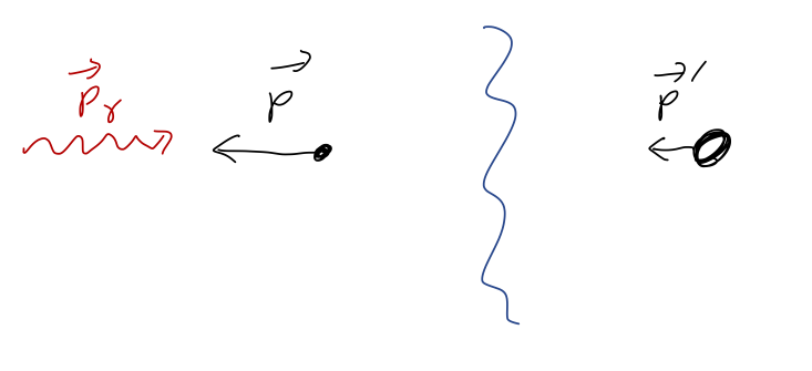
- Laser cooling and laser sails: you'll recall from classical mechanics that photons carry momentum, \( p = h/\lambda \). Although we've only proved it for Newtonian mechanics, momentum conservation actually holds down to the most fundamental theories we know of! So we can understand the idea of laser cooling: if we shine a laser on an atom at the right frequency, the atom can absorb the photon. When it does, momentum conservation tells us that the atom has to slow down. At a larger scale, a laser sail works by shining a laser at a highly reflective surface. The photons bounce off in the opposite direciton, pushing the sail forward according to momentum conservation. This is a promising method of propulsion for very small spacecraft.
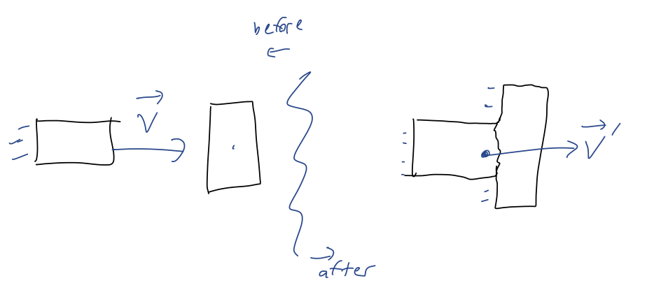
- Explosions: something like a firework detonation, or a rocket separating off one of its stages. Again, the internal forces involved here can be complicated and violent, but nevertheless momentum conservation constrains the combined motion of all the pieces. If we track N-1 pieces after the explosion, we know exactly the trajectory of the last piece.
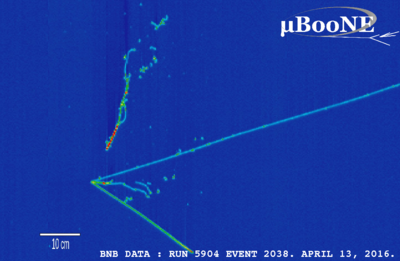
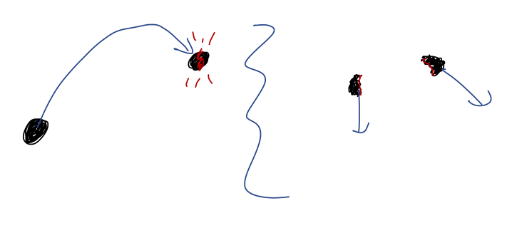
- Invisible particles: this is really just another explosion example, but it's an interesting one! The study of subatomic particles makes heavy use of momentum conservation. The picture above, from the MicroBooNE experiment at Fermilab, shows visible tracks for charged particles passing through their detector. However, notice that all of the tracks point back to a single point, and if we try to add up the total momentum it's definitely pointing to the right. We can thus infer that there was an incoming particle that is invisible to our detector, which collided at the vertex where the tracks meet and caused the visible particles to fly off. (In fact, this invisible particle is a neutrino, and is precisely the particle that the MicroBooNE experiment was designed to look for.) This is cutting-edge research, but we don't need to know any details of particle physics to understand the basic idea, just momentum conservation!