Let's finish our discussion of rocket propulsion with a couple more examples.
Example: rocket car
Suppose we have a rocket-powered car moving in a straight line across a flat surface. Ignoring friction and air resistance, how does the position of the car change with time?
As always we start with the equation of motion, which is
\[ \begin{aligned} m(t) \ddot{x} = F_{\rm thrust}. \end{aligned} \]
This looks simple, but we have to deal with the extra complication that \( m(t) \) is time dependent. Fortunately, since we know that the mass ejection rate is constant, it's easy to see that
\[ \begin{aligned} m(t) = m_0 - kt. \end{aligned} \]
Our equation of motion is nice and separable: moving things around and integrating, we find first that
\[ \begin{aligned} \int d\dot{x} = F_{\rm thrust} \int \frac{dt}{m_0 - kt} \\ \dot{x}(t) = \dot{x}(0) - \frac{F_{\rm thrust}}{k} \ln \left(1 - \frac{kt}{m_0}\right). \end{aligned} \]
Integrating one more time, and using the result \( \int dx \ln x = x \ln x - x \) (which is easy to verify), we have
\[ \begin{aligned} x(t) = x(0) + \left(\dot{x}(0) + \frac{F_{\rm thrust}}{k} \right) t + \frac{F_{\rm thrust} (m_0 - kt)}{k^2} \ln \left(1 - \frac{kt}{m_0}\right). \end{aligned} \]
This is an analytic solution, but it's already pretty complicated - and this was the simplest possible case, with no other forces acting! It's also worth noting that this solution is not valid for all times: mathematically, we can see that at \( t = m_0 / k \) the log blows up, and we have \( x(m_0 / k) \rightarrow \infty \)!
Of course, \( t = m0 / k \) is the time at which \( m(t) = 0 \), which is obviously not possible. Physically, we know that our solution is only valid until the fuel is burned completely, at which point \( F{\rm thrust} \) shuts off and we just have constant speed from that point on (the speed we already found with the rocket equation above, in fact.)
What if we have other external forces? If we wanted to track the motion of the rocket-exhaust system combined, we could keep track of the combined center of mass and see how the forces act on that. However, this would be complicated to do! Fortunately, we don't care about the combined system - we only care about the net forces on the rocket itself. So if we have additional forces like drag or gravity, we just treat them as acting on the rocket, in addition to the thrust force provided by the ejected mass.
For example, taking both forces above at once and assuming quadratic drag, a rocket moving vertically from the Earth's surface has the equation of motion
\[ \begin{aligned} m(t) \dot{v} = \vec{F}_{\rm thrust} - m(t) g - cv^2. \end{aligned} \]
although this will get more complicated quickly if we remember that the density of air depends strongly on altitude, so \( c = c(z) \) for a more realistic model (and at some point, \( g \) also depends on position.) This also means there's no terminal velocity for a rocket launch into space; once it gets out of the Earth's atmosphere and away from the Earth's gravity, the rocket will just continue to move at constant speed.
As you can start to see, getting much further with practical examples of rocketry is going to require a lot of additional details, and the equations will become difficult to handle very, very quickly. Basically, any realistic rocket problems are going to involve heavy use of numerical solutions. However, there's one more interesting example that we can do, which is to consider the idea of a multi-stage rocket.
Example: multi-stage rockets
Ignoring all other forces (e.g. imagine we're working in deep space), let's compare the maximum speed of two different rockets. Rocket A is simple rocket with a fuel-to-mass ratio of \( m_{A,F} / m_{A,E} = 25 \). Rocket B is a two-stage rocket, which means it's two rockets stuck together: both stage 1 and stage 2 have a fuel-to-mass ratio of \( m_{B1,F} / m_{B1,E} = m_{B2,F} / m_{B2,E} = 10 \). Stage 2 is also about 5 times lighter than stage 1, i.e. \( m_{B1,E} / m_{B2,E} = 5 \). Assuming \( v_{\rm exh} = 2.5 \) km/s, what is the \( \Delta v \) supplied by each rocket?
We only need one equation here, although we'll need it a few times. From above, we can get the \( \Delta v \) for rocket A just by plugging in:
\[ \begin{aligned} (\Delta v)_A = |v_{\rm exh}| \log \left(1 + 25 \right) = 8.1\ {\rm km} / {\rm s} \end{aligned} \]
For the two-stage rocket, we have to be more careful what masses we plug in. Working in units of \( m_{B2,E} \equiv m \), we have for the first stage \( m_{B1,E} = 5m \) and thus
\[ \begin{aligned} m_F = 10 m_{B1,E} = 50m \\ m_E = m_{B1,E} + m_{B2,F} + m_{B2,E} = (5 + 10 + 1) = 16m \end{aligned} \]
so after the first-stage burn,
\[ \begin{aligned} (\Delta v)_{B1} = |v_{\rm exh}| \log \left(1 + \frac{50}{16} \right) = 3.5\ {\rm km} / {\rm s} \end{aligned} \]
Now we discard the first stage and just consider the second stage alone, which is much easier to plug in for:
\[ \begin{aligned} (\Delta v)_{B2} = |v_{\rm exh}| \log \left(1 + 10\right) = 6.0\ {\rm km} / {\rm s} \end{aligned} \]
So in total, the second rocket achieves
\[ \begin{aligned} (\Delta v)_B = 9.5\ {\rm km}/{\rm s}, \end{aligned} \]
somewhat better than rocket A - despite the fact that the individual stages had a much lower fuel-to-mass ratio! Qualitatively, this makes sense: if we can dump some of the mass of our rocket partway through, then the fuel-to-mass ratio at that point is immediately improved. (After the first-stage burn but before separation, our fuel-to-mass ratio is all the way down to 1.7.)
By the way, 25 to 1 is generally considered about the best possible ratio for a single rocket stage, based on available technology for both rocket fuels and engineering the rocket itself. The ratio of 5 in mass between the two stages is taken from SpaceX's Falcon 9 rocket, but the real Falcon 9 has much better single-stage performance, with 18:1 for the first stage and 25:1 for the second. This gives the Falcon 9 an approximate \( \Delta v \) of 12.1 km/s (before including a payload) - plenty to make it not just off the Earth, but all the way to Mars!
Angular momentum
Before we move on to energy, let's have a brief look at angular momentum. The definition of angular momentum is
\[ \begin{aligned} \vec{\ell} = \vec{r} \times \vec{p} = m\vec{r} \times \dot{\vec{r}} \end{aligned} \]
for a point mass. It's very important to stress that, unlike linear momentum, this depends strongly on what the origin of our coordinate system is! Consider the following example: we have a 1 kg mass moving in a straight line at \( v = 2 \) m/s. Here's a sketch with two possible coordinate systems:
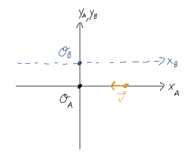
The linear momentum of the particle is the same in both coordinate systems, \( \vec{p} = (-2,0,0)\ {\rm kg} \cdot {\rm m} / {\rm s} \). However, the angular momentum is different:
\[ \begin{aligned} \vec{\ell}_A = \vec{r}_A \times \vec{p} = (4,0,0) \times (-2, 0, 0) = (0,0,0)\ {\rm kg} \cdot {\rm m}^2 / {\rm s} \\ \vec{\ell}_B = \vec{r}_B \times \vec{p} = (4, -2, 0) \times (-2, 0, 0) = (0,0,-4)\ {\rm kg} \cdot {\rm m}^2 / {\rm s} \end{aligned} \]
(check the direction with the right-hand rule!) Of course, this isn't really a fundamental difference: if I set up a third coordinate system with origin \( \mathcal{O}_C \) which is moving to the left at 2 m/s, then the linear momentum will change to \( \vec{p}_C = (0,0,0) \). Momentum is something that we define to make sense of a physical system, but all that really matters is the actual motion is the same no matter what coordinates we choose. (I stress this point here because it often catches people off-guard that angular momentum can change even if your coordinates aren't moving.)
In the presence of forces, \( \vec{p} \) will change, and therefore \( \vec{L} \) can also be changed by forces. To see exactly how, we just take the time derivative:
\[ \begin{aligned} \frac{d\vec{\ell}}{dt} = m\frac{d}{dt} \left(\vec{r} \times \dot{\vec{r}} \right) \\ = m \dot{\vec{r}} \times \dot{\vec{r}} + m \vec{r} \times \ddot{\vec{r}} \\ = \vec{r} \times \vec{F}, \end{aligned} \]
where on the last line the first term vanished since it's the cross product of a vector with itself, and in the second term we plugged in Newton's second law. This cross product of distance and force is called the torque,
\[ \begin{aligned} \vec{\Gamma} \equiv \vec{r} \times \vec{F}. \end{aligned} \]
(Some references will use \( \tau \) instead of \( \Gamma \) for torque, so beware.) This gives us a rotational version of Newton's second law,
\[ \begin{aligned} \vec{\Gamma} = \frac{d\vec{\ell}}{dt}. \end{aligned} \]
Conservation of angular momentum
We can identify a new conservation law from the last equation we wrote above: if there is no net torque on a point mass, \( \vec{\Gamma} = 0 \), then angular momentum is conserved - \( d\vec{\ell} / dt = 0 \). Note that this can be true even if there is a net force, as long as \( \vec{r} \times \vec{F} = 0 \).
Of course, this isn't very useful for a single point mass! There are not many situations where there is a net force but no torque for the entire motion of a single particle, just because \( \vec{r} \) will generally change with time. The good news is that like conservation of linear momentum, this law also applies to collections of masses. Breaking out our trusty set of \( N \) point masses \( {m_\alpha } \), it can be shown that if we define the total angular momentum
\[ \begin{aligned} \vec{L} \equiv \sum_{\alpha=1}^N \ell_\alpha, \end{aligned} \]
then \( \dot{\vec{L}} = 0 \) if the net external torque is zero, and more generally,
\[ \begin{aligned} \vec{\Gamma}_{\rm ext} = \frac{d\vec{L}}{dt}. \end{aligned} \]
(I am not going to do the proof in class - it's another round of sums, but this time with cross products added in. Taylor shows this result in chapter 3.5, and I encourage you to have a look.)
As with conservation of linear momentum, a nice application of this conservation law is learning things about horribly complicated systems, so long as they have no external torques acting on them. The formation of the solar system, for example, was a horribly messy and complicated process spanning billions of years. However, from the simple fact that the planets currently have a net angular momentum (all of the orbits go the same way, which is the same way the Sun is spinning!), we know that whatever primordial structure the solar system formed from must have been spinning, and we can even relate its rotational speed to its size!
This is especially useful in combination with the center of mass (CM)! It turns out that for any extended object, we can decompose its motion into two parts: the motion of the CM itself, treating it like a point particle, and then rotation of the object about the CM. The latter subject is fairly complicated, but you'll see it worked out in detail next semester, and it's much, much easier to study rotation using the CM of an object instead of using an arbitrary set of coordinates.
There are a couple of immediate applications that we could try to work through - Taylor shows a few examples, including a version of Kepler's second law. But these are specialized examples, especially the planetary motion one, and I think it's better to put them off until you're really prepared to tackle the problem of rotation and angular momentum in full. So we'll end the chapter here.