Our next big physics topic will be energy. Energy also satisfies a conservation law, like momentum and angular momentum. However, energy is much more subtle; as Taylor points out, a lot of confusion tends to come from the fact that energy comes in many different forms, whereas there's only one kind of (linear or angular) momentum. This will also lead us naturally into our next big math topic, which is vector calculus.
Since this is a mechanics class, we'll start with kinetic energy, which is energy associated with motion. For a point mass, the kinetic energy \( T \) is given by the formula
\[ \begin{aligned} T = \frac{1}{2} mv^2. \end{aligned} \]
You'll notice right away that like linear momentum, energy is not independent of our choice of coordinates; if I choose a moving coordinate system, then \( v \) will change and so will \( T \). So in and of itself, energy is not some immutable property of an object; it's a useful construct that will help us solve for the motion.
To better understand the physical meaning of energy, let's try to connect it to Newton's laws. We start by just taking a time derivative to see what happens. To do this properly, we should be careful and remember that \( v^2 \) is really \( \vec{v} \cdot \vec{v} \), so the derivative is:
\[ \begin{aligned} \frac{dT}{dt} = \frac{m}{2} \frac{d}{dt} \left( \vec{v} \cdot \vec{v} \right) \\ = \frac{m}{2} \left( \vec{v} \cdot \dot{\vec{v}} + \dot{\vec{v}} \cdot \vec{v} \right) \\ = m \vec{v} \cdot \dot{\vec{v}} \\ = \frac{d\vec{r}}{dt} \cdot \vec{F}_{\rm net}, \end{aligned} \]
using Newton's second law at the end, and I wrote out the time derivative to make things look more symmetric. So the change in kinetic energy is given by the dot product of applied force with the velocity, which seems interesting but isn't really enlightening yet.
Now suppose that we're interested in what is happening to our system during an infinitesmal time interval \( dt \). We can multiply both sides by \( dt \) to find the equation
\[ \begin{aligned} dT = \vec{F}_{\rm net} \cdot d\vec{r} \equiv dW_{\rm net} \end{aligned} \]
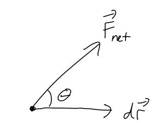
where the right-hand side defines the infinitesmal work, \( dW \). Let's make a couple of useful observations about \( dW \) before we move on to integrating it, all of which apply to work in general. First of all, notice that \( dW \) is a scalar since it comes from a dot product. In fact, we can rewrite it using one of our dot-product identities as
\[ \begin{aligned} dW_{\rm net} = F_{\rm net} dr \cos \theta. \end{aligned} \]
It's important to emphasize a few special cases that can be counter-intuitive:
- \( dW_{\rm net} \) can be zero, even if \( F_{\rm net} \) is non-zero. (From above, this happens when \( \theta = 90^\circ \), i.e. when \( \vec{F}_{\rm net} \) is perpendicular to \( dr \).)
- \( dW_{\rm net} \) can be negative, if \( F_{\rm net} \) and \( d\vec{r} \) point in opposite directions. (A simple example is a particle which is decelerating, so the net force is opposite its direction of motion.)
If we integrate both sides as our mass moves from point \( \vec{r}_1 \) to point \( \vec{r}_2 \), then we find the result
\[ \begin{aligned} T_2 - T_1 = \int_{\vec{r}_1}^{\vec{r}_2}\ dW_{\rm net} = \int_{\vec{r}_1}^{\vec{r}_2}\ d\vec{r} \cdot \vec{F}_{\rm net}, \end{aligned} \]
or more compactly, if we call the result of the integral over \( dW_{\rm net} \) as just \( W_{\rm net} \) (the net work), then
\[ \begin{aligned} \Delta T = W_{\rm net} \end{aligned} \]
which is known as the "work-KE theorem". This is an important relationship, because it gives us a way to interpret what kinetic energy actually means physically.
Before we move on to interpretation, a brief comment on my notation above. It's important to emphasize that the work-KE theorem is only true for a single point mass, and that it's only true if we use the net force. However, it's often useful to define the work done by a single force, which we can do using the same equation,
\[ \begin{aligned} W = \int_{\vec{r}_1}^{\vec{r}_2} d\vec{r} \cdot \vec{F}. \end{aligned} \]
Since \( d\vec{r} \cdot \vec{F}_{\rm net} \) splits apart into \( d\vec{r} \cdot \vec{F}_1+ d\vec{r} \cdot \vec{F}2 + ... \) in the case of multiple forces, the work also splits apart neatly, \( W{\rm net} = W_1 + W_2 + ... \).
What we can see from this result is that changes in kinetic energy tell us something about the overall motion of a physical object. Although we can calculate \( T \) for an object at any moment in time, the significance of \( T \) is that it summarizes the history of how our object has moved. If our object starts from rest, the value of \( T \) later on is related to the sum total of all of the net forces acting in the direction of its path.
Thinking in the opposite direction, for an object which starts in motion, \( T \) also measures its capability of supplying a force later. Remember the Mythbusters problem from the homework, where we had to calculate the force applied by a penny coming to a stop? The solution I gave was to assume a constant force \( F = m\dot{v} \), solve for the stopping time
\[ \begin{aligned} t_s = \frac{mv_0}{F} \end{aligned} \]
and then plug in to find the stopping distance,
\[ \begin{aligned} d(t_s) = v_0 t_s - \frac{1}{2} \frac{F}{m} t_s^2 = \frac{mv_0^2}{2F}. \end{aligned} \]
But you probably recognize what's happening here already: I can rewrite this as
\[ \begin{aligned} F d(t_s) = \frac{1}{2} mv_0^2 \end{aligned} \]
which is just \( W_{\rm net} = \Delta T \)! Instead of solving for the details of the motion, we could have found the force applied by the stopping penny in one line by using the work-KE theorem. Hopefully, you're starting to see how energy is both tricky to define, and very useful to work with!
Before we can continue our study of work and kinetic energy, we have to deal with an important question: how do we evaluate the integral for work in general? Having another look at it:
\[ \begin{aligned} W_{\rm net} = \int_{\vec{r}_1}^{\vec{r}_2} \vec{F}_{\rm net} \cdot d\vec{r} \end{aligned} \]
How do we interpret this integral, where the integration variable is a vector? The best way to understand what this expression means is to go back to the infinitesmal picture for \( dW \), and imagine building up the whole integral by just stringing together infinitesmal pieces:
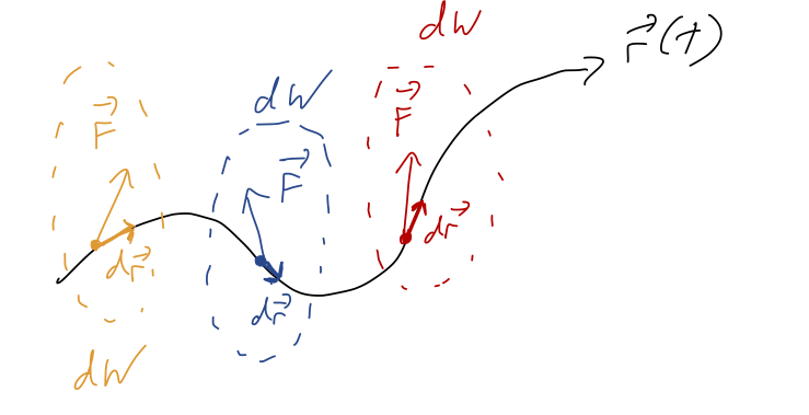
So the integral for \( W \) is a sum along the path traced out by \( \vec{r} \).,
\[ \begin{aligned} W = \sum_i dW_i \rightarrow \int dW \end{aligned} \]
where the sum becomes an integral as we make our steps along the trajectory \( d\vec{r} \) smaller and smaller. Notice that this is not the "area under the curve" or anything related to it; we're summing up the dot products \( \vec{F}_{\rm net} \cdot d\vec{r} \) as we follow the curve. This is an example of a line integral.
Before we get into the formalism of line integrals, let's warm up with a few simple physics examples. There's one special case where we already know how to do the integral: if the motion is one-dimensional. For one-dimensional motion, all vectors have only one component, so the dot product is trivial. If we call our single direction \( x \), then
\[ \begin{aligned} W_{1d} = \int_{x_1}^{x_2} \vec{F}_{\rm net}(x) \cdot d\vec{x} \end{aligned} \]
and better still, if the net force is constant,
\[ \begin{aligned} W_{1d} = \vec{F}_{\rm const} \cdot \int_{x_1}^{x_2} dx = \vec{F}_{\rm const}\ \cdot \Delta \vec{x}. \end{aligned} \]
(I'm keeping the dot product notation to remind us that the directions still matter in one dimension, so we can get minus signs here.)
Now the physics examples. Before you read my solution, think about it yourself: what do you expect the net work to be in each example? Can you estimate it yourself first? Does the result you get from the math make sense?
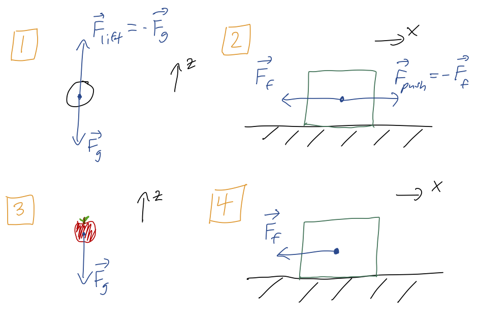
Example 1: you lift a mass into the air at constant speed, up to a height \( h \).
\[ \begin{aligned} W_g = \vec{F}_{\rm g} \cdot \Delta \vec{z} = (-mg \hat{z}) \cdot (+h\hat{z}) = -mgh \\ W_{\rm lift} = \vec{F}_{\rm lift} \cdot \Delta \vec{z} = (+mg \hat{z}) \cdot (+h \hat{z}) = +mgh \end{aligned} \]
Equal and opposite, so \( W_{\rm net} = Wg + W{\rm you} = 0 \) - easy to see since \( \vec{F}_{\rm net} = 0 \) too. Since the speed is constant, we also immediately see that \( \Delta T = 0 \).
Example 2: you push a box along a floor with friction, again at constant speed, for a distance \( d \).
\[ \begin{aligned} W_f = \vec{F}_f \cdot \Delta \vec{x} = (-\mu_k mg \hat{x}) \cdot (+d \hat{x}) = -\mu_k mgd \\ W_{\rm push} = \vec{F}_{\rm push} \cdot \Delta \vec{x} = (+\mu_k mg \hat{x}) \cdot (+d \hat{x}) = +\mu_k mgd \end{aligned} \]
Once again, \( W_{\rm net} = 0 \) since the net force is zero, and since the speed is constant once again \( \Delta T = 0 \). This is basically the same as the first example, but it's important to see that friction is no different from gravity. We often think of friction as a "dissipative force", one that doesn't conserve energy - but it still obeys the work-KE theorem.
Just to emphasize the point, note the difference between your work and net work. Although the net work is zero, you are doing work in order to push the box against friction. (This matches your physical intuition - if you push a heavy box, you certainly feel like you're doing work!)
Example 3: an apple falls out of a tree from height \( h \).
This isn't quite the same as example 1, because now the apple is moving down instead of up. If we calculate the work out again,
\[ \begin{aligned} W_g = \vec{F}_{\rm g} \cdot \Delta \vec{z} = (-mg \hat{z}) \cdot (-h\hat{z}) = +mgh. \end{aligned} \]
This is also the net work, since there's only one force this time. So by the work-KE theorem, we expect \( \Delta T = mgh \). If the apple starts from rest, then
\[ \begin{aligned} \Delta T = \frac{1}{2} mv_f^2 = mgh \rightarrow v_f = \sqrt{2gh} \end{aligned} \]
which you can easily confirm is exactly the speed you'll find just solving \( \ddot{z} = -g \) for the speed when \( z=-h \). (But just using work-KE is a lot less algebra to find \( v_f \)!)
Example 4: the box from example 2 is released at speed \( v_0 \), and slides to a stop over distance \( D \) due to friction.
This is just example 2 without the pushing force, since the box is continuing to move forwards. The work done by friction is therefore still \( W_f = -\mu_k mgD \). Using work-KE, we have
\[ \begin{aligned} \Delta T = 0 - \frac{1}{2} mv_0^2 = -\mu_k mgD \rightarrow v_0 = \sqrt{2\mu_k g D} \end{aligned} \]
allowing us to find the initial speed based on the stopping distance, for example. In fact, this is basically the same solution as example 3, since the frictional force is constant. Again, this is here to emphasize that in terms of work and kinetic energy, there are no exceptions to the work-KE theorem!
Line integrals
Let's come back to the general equation for work in three dimensions,
\[ \begin{aligned} W = \int_{\vec{r}_1}^{\vec{r}_2} \vec{F} \cdot d\vec{r}. \end{aligned} \]
This is an example of a line integral. To see why this is tricky to evaluate, let's pick a concrete example in two dimensions. Suppose that we have a constant force of the form
\[ \begin{aligned} \vec{F} = Fx\hat{x} + 2F\hat{y}, \end{aligned} \]
and we'd like to compute the work from \( \vec{r}_1 = (0,0) \) to \( \vec{r}_2 = (2,1) \). How do we interpret the vector differential \( d\vec{r} \)? We already know that derivatives of vectors are simple to evaluate: we just take the derivative of each component. Similarly, \( d\vec{r} \) just means we have a differential length in each component. In Cartesian coordinates,
\[ \begin{aligned} d\vec{r} = dx \hat{x} + dy \hat{y} + dz \hat{z}. \end{aligned} \]
So in our example, we can evaluate the dot product to find
\[ \begin{aligned} W = \int_{\vec{r}_1}^{\vec{r}_2} (Fx dx + 2F dy). \end{aligned} \]
The appearance of two differentials at once, \( dx \) and \( dy \), signals that we can't just evaluate this integral normally yet. More importantly, we have to specify one more thing not written down, which is the path along which we want to evaluate this integral. This is one of the sloppy things about this notation, although it's used commonly: there are infinitely many ways to get from \( \vec{r}_1 \) to \( \vec{r}_2 \)!
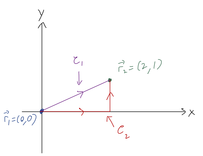
Notice that these are directed paths, hence the arrows; just like a regular integral, if we go backwards (reverse the limits of integration so we move from \( \vec{r}_2 \) to \( \vec{r}_1 \)), then we get an extra minus sign.
In math books, the integral will often be written instead as
\[ \begin{aligned} W = \int_\mathcal{C} \vec{F} \cdot d\vec{r}, \end{aligned} \]
where \( \mathcal{C} \) denotes a curve - the entire path we take, along with its endpoints. In physics applications, when we do the work integral, the curve is always \( \vec{r}(t) \), the trajectory followed by our point mass.
Next time, we'll dig deeper into how to evaluate line integrals.