To recap briefly: when faced with a line integral, we need to work through the following steps to find the answer:
- Choose vector coordinates and find \( \vec{F} \cdot d\vec{r} \). (The form of \( \vec{F} \) is usually most important in coordinate choice, but don't ignore the path completely.)
- Parameterize the path, writing it in terms of a single coordinate or parameter.
- Use the results of 1) and 2) to write the work integral as a regular integral over our single parameter.
- Do the integral and find the answer!
I skipped the example below in class since we just did a line integral tutorial, but if you'd like some extra practice, give it a try before you look at my solution!
Example: another line integral
Calculate the work integral \( W = \vec{F} \cdot d\vec{r} \) for the force \( \vec{F} = 2\vec{r} \) and parabolic path \( x = 1-y^2 \), from \( (1,0) \) to \( (0,1) \).
Let's start by sketching the path:
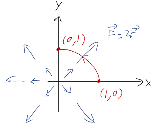
It might be tempting to choose polar coordinates since the force field is radial, but radial force is pretty easy to describe in Cartesian coordinates too, and our path will be easier in Cartesian. (If we had a force in the \( \hat{\phi} \) direction, we'd almost certainly want polar instead!) Using Cartesian, we have
\[ \begin{aligned} \vec{F} = 2x \hat{x} + 2y \hat{y} \end{aligned} \]
and so
\[ \begin{aligned} \vec{F} \cdot d\vec{r} = 2Fx dx + 2Fy dy. \end{aligned} \]
Next, we parameterize the path. Here \( y \) itself is a nice parameter, since we already have the path written in the form \( x = 1-y^2 \). In terms of differentials, we have
\[ \begin{aligned} dx = -2y dy \end{aligned} \]
and in terms of \( y \), our path begins at \( y=1 \) and ends at \( y=0 \). So writing out our line integral,
\[ \begin{aligned} W = \int \vec{F} \cdot d\vec{r} = \int (2Fx dx + 2Fy dy) \\ = 2F \int_1^0 (1-y^2) (-2y dy) + y dy \\ = 2F \int_1^0 dy\ (-y + 2y^3) \\ = 2F \left. \left(-\frac{y^2}{2} + \frac{y^4}{2} \right) \right|_0^1 \\ = 0. \end{aligned} \]
Although the work is exactly zero here, it's sort of a coincidence: we notice that the cancellation of \( y^2 \) and \( y^4 \) only worked at \( y=0 \) and \( y=1 \), so pretty much any other starting or ending points along this curve would yield non-zero work.
Potential energy
Now that we know how to calculate line integrals, let's go back to the physical meaning of work. In mechanics, we aren't going to be dealing with completely arbitrary paths; the work-KE theorem only applies to the path which results from Newton's laws and whatever forces are applied.
At the beginning of this section, I mentioned that energy comes in many forms. To really see how work and energy can be useful, we need to introduce a second form of energy, which is called potential energy. You may remember the buzzwords from intro physics: a potential energy can only be defined for a conservative force. This turns out to be a consequence of how we define a conservative force, acting on a point mass:
- Conservative forces depend only on \( \vec{r} \) and constants.
- The work done by a conservative force from \( \vec{r}_1 \) to \( \vec{r}_2 \) is independent of the path taken.
When both of these properties are satisfied, if we're given two points anywhere in space, we immediately know the work done by the conservative force when we move from one to the other. (Property 1 matters because we don't need any extra info to decide the work done, like how long it took to move between the points or how fast the object was moving.)
Now let's pick a special point \( \vec{r}_0 \) somewhere in space and hold it fixed. The work done to get to any other point \( \vec{r} \) from this special point is a function only of where the second point is:
\[ \begin{aligned} W_{\vec{r}_0 \rightarrow \vec{r}} = \int_{\vec{r}_0}^{\vec{r}} \vec{F} \cdot d\vec{r} = -U(\vec{r}) \end{aligned} \]
This defines the potential energy function. (It only depends on \( \vec{r} \), because we've agreed to hold \( \vec{r}_0 \) fixed.) The minus sign I added at the end is extremely important, as we'll see below! Basically, it has to do with energy conservation: positive work will give a positive change in kinetic energy, which will be compensated by a negative change in potential energy so the total stays fixed.
Now, let's do a short mathematical proof that will let us make two nice observations. If we try to calculate \( U(\vec{r}_0) \), we find the following:
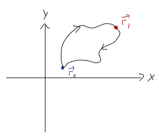
\[ \begin{aligned} U(\vec{r}_0) = -\int_{\vec{r}_0}^{\vec{r}_0} \vec{F} \cdot d\vec{r} \\ = -\int_{\vec{r}_0}^{\vec{r}_1} \vec{F} \cdot d\vec{r} - \int_{\vec{r}_1}^{\vec{r}_0} \vec{F} \cdot d\vec{r} \end{aligned} \]
where I'm now just picking another arbitrary point \( \vec{r}_1 \) and using the properties of definite integration to split it up. Okay, this isn't a normal integral. Really, the original line integral represents a closed path from \( \vec{r}_0 \) back to itself, and I've picked a point somewhere along that path and divided it in half:
Reversing the limits of any integral, including a line integral, just gives us a minus sign:
\[ \begin{aligned} U(\vec{r}_0) = -\int_{\vec{r}_0}^{\vec{r}_1} \vec{F} \cdot d\vec{r} + \int_{\vec{r}_0}^{\vec{r}_1} \vec{F} \cdot d\vec{r} = 0. \end{aligned} \]
These two integrals are on two different curves, but since \( \vec{F} \) is conservative it doesn't matter; their results are equal and they cancel. The first nice observation is that picking a reference point is the same thing as choosing where our potential energy function is equal to zero, which you'll remember as something you can do with e.g. the gravitational potential.
If you choose a different reference point \( \vec{r}'_0 \), then your potential energy function will be different, but in a simple way:
\[ \begin{aligned} U'(\vec{r}) = -\int_{\vec{r}'_0}^{\vec{r}} dW = -\int_{\vec{r}'_0}^{\vec{r}_0} dW - \int_{\vec{r}_0}^{\vec{r}} dW \\ = U(\vec{r}_0') - U(\vec{r}) \end{aligned} \]
or in other words, the difference between \( U \) and \( U' \) is just a shift by a constant.
The second nice observation we can make is that we've just showed that for any force which satisfies property 2 above (work done is path-independent), the work done around a closed path is exactly zero. You may remember the special notation for closed-path integrals from vector calculus:
\[ \begin{aligned} \oint \vec{F} \cdot d\vec{r} = 0. \end{aligned} \]
If you remember that notation, you probably also remember that \( \vec{F} \cdot d\vec{r} \) shows up in a very powerful result called Stokes' theorem. We'll come back to that later on: it will give us a much clearer picture of why a force would obey property 2 above, which seems sort of arbitrary right now.
In fact, conditions 1 and 2 seem fairly specialized, and they are. We'll put condition 2 aside for now, but there are many familiar examples of forces that violate the first condition:
- Air resistance (depends on \( \vec{v} \))
- Magnetic force (depends on \( \vec{v} \))
- A time-varying electric field (depends on \( t \))
- Normal force (sometimes depends on \( \vec{v} \), or on \( \vec{r} \), or on \( m(t) \)...)
- Friction (sometimes depends on the direction of \( \vec{r} \), plus same problems as normal force)
If you just consider motion for which the direction of movement is constant, then friction can temporarily look okay under condition 1. However, it will always violate condition 2: the frictional force is just constant, so its work done is \( |\vec{F}| L \) over a path of length \( L \), which means it matters which path we take.
Back to our potential energy \( U \). Assuming for the moment that \( \vec{F} \) is the only force acting, the work-KE theorem applies:
\[ \begin{aligned} T(\vec{r}_2) - T(\vec{r}_1) = W_{1 \rightarrow 2} = \int_{\vec{r}_1}^{\vec{r}_2} \vec{F} \cdot d\vec{r} = -U(\vec{r}_2) + U(\vec{r}_1) \end{aligned} \]
or rearranging,
\[ \begin{aligned} T(\vec{r}_1) + U(\vec{r}_1) = T(\vec{r}_2) + U(\vec{r}_2). \end{aligned} \]
In other words, the combination
\[ \begin{aligned} E = T + U, \end{aligned} \]
which we call the mechanical energy (or just "the energy"), doesn't change as we move from \( \vec{r}_1 \) to \( \vec{r}_2 \). Since this is true for any two points we choose, and since the path and other variables can't change the work, we see that in the presence of a conservative force, energy is conserved:
\[ \begin{aligned} \frac{dE}{dt} = 0. \end{aligned} \]
Since we used the work-KE theorem, we technically assumed above that \( \vec{F} \) is the only force acting in our system. If we have multiple forces, remember that we can divide net work up into the sum of work due to each individual forces. If they're all conservative, then we can write a separate potential energy function for each force. So the more general version of the mechanical energy is
\[ \begin{aligned} E = T + U_1 + U_2 + U_3 + ... \end{aligned} \]
if we have several forces \( \vec{F}_1, \vec{F}_2, \vec{F}_3... \)
Of course, as we just noted there are plenty of non-conservative forces around. The work-KE theorem still applies to them, and we can still split them up. If we have both conservative and non-conservative forces, then
\[ \begin{aligned} \Delta T = W_{\rm net} = W_{\rm cons} + W_{\rm non-cons} \\ = -\Delta U + W_{\rm non-cons} \end{aligned} \]
or
\[ \begin{aligned} \Delta E = W_{\rm non-cons} \end{aligned} \]
So energy is not conserved if we have non-conservative forces, but we know exactly how it will change if we keep track of the work done by those forces.
A note about the deeper interpretation of this: friction and air resistance are not fundamental forces: ultimately, they come from electromagnetic forces between the atoms in our object and the surface or medium providing the force. All of the known fundamental forces of nature are conservative, which means that total energy is conserved, period. When we find a non-zero \( \Delta E \) due to something like friction, that "lost" energy is just being transferred into another form - mostly heat, in the case of friction.
One more brief aside, about magnetic fields - which are sort of a weird example. They are non-conservative because they depend on speed, but they also don't do any work at all because the magnetic force is always perpendicular to \( \vec{v} \)! So a system including a magnetic field will still conserve mechanical energy - but we can't write a potential energy function to describe the motion. (In other words, conserving energy alone isn't sufficient for a force to be "conservative" by the definition we're using.)
At this point, Taylor does an example of mixing conservative and non-conservative forces, involving a sliding block with friction. We solved the sliding block with friction way back in chapter 1, but work gives a quicker way to find the speed as a function of the height of the block. I'll skip this example because Taylor already did it, and unfortunately there aren't any other good simple examples of this sort of thing: you could try to do a similar trick with linear air resistance, but the equations are unsolvable and you have to resort to numerics anyway, so using energy and work doesn't really help.
Force from the potential
Let's come back to the relationship between potential energy and force. We defined the potential based on a path integral of the force:
\[ \begin{aligned} U(\vec{r}) = -\int_{\vec{r}_0}^{\vec{r}} \vec{F} \cdot d\vec{r}, \end{aligned} \]
which uses \( \vec{F} \) to find \( U \). But we know that regular integrals can be inverted using derivatives, so it's natural to ask: can we go the other way here as well, i.e. can we find \( \vec{F}(\vec{r}) \) given \( U(\vec{r}) \)?
The answer is yes, and the easiest way to see it is thinking about the infinitesmal version of the integral above. Remember that a line integral is just a sum over lots of infinitesmal segments, which means that we can go backwards and notice that an infinitesmal contribution to the potential energy takes the form
\[ \begin{aligned} dU = -\vec{F} \cdot d\vec{r} \end{aligned} \]
(you can think of this as the change in potential if we move \( \vec{r} \) by a tiny amount; also, we get the formula above back by integrating both sides.) There's another way to write out \( dU(\vec{r}) \); by using the chain rule with respect to the individual coordinates, we have
\[ \begin{aligned} dU = \frac{\partial U}{\partial x} dx + \frac{\partial U}{\partial y} dy + \frac{\partial U}{\partial z} dz. \end{aligned} \]
We can write out the first version of \( dU \) in a very similar way by expanding the dot product:
\[ \begin{aligned} dU = -F_x dx - F_y dy - F_z dz \end{aligned} \]
These equations are both \( dU \), so their right-hand sides have to be equal. But more than that, they have to be equal for any possible path that we choose! Changing a path will change how \( dx \), \( dy \), and \( dz \) vary, which means that for these equations to always be true, the things multiplying \( dx \), \( dy \), and \( dz \) must be equal. This gives us the result
\[ \begin{aligned} \vec{F} = -\frac{\partial U}{\partial x} \hat{x} - \frac{\partial U}{\partial y} \hat{y} - \frac{\partial U}{\partial z} \hat{z} \end{aligned} \]
or written more compactly,
\[ \begin{aligned} \vec{F} = -\vec{\nabla} U \end{aligned} \]
where \( \vec{\nabla} \) represents the gradient of the function \( U \). (The upside-down triangle symbol is usually called 'del', although another common name is 'nabla', which comes from the Greek word for 'harp'.) The gradient can be thought of as being defined through the equation
\[ \begin{aligned} \vec{\nabla} \equiv \frac{\partial}{\partial x} \hat{x} + \frac{\partial}{\partial y} \hat{y} + \frac{\partial}{\partial z} \hat{z} \end{aligned} \]
in Cartesian coordinates. Clearly from the way we found it, \( \vec{\nabla} \) acts as the inverse operation to a regular line integral, just as an ordinary derivative is the inverse of an ordinary integral. (Because it is a vector, \( \vec{\nabla} \) will look different if we change coordinates! I won't go through those formulas for now, just warn you that it will happen.)
If you have more of a formal math background, you might recognize \( \vec{\nabla} \) as a sort of object called an operator. An operator is basically a map from one class of objects to another. In this case, it takes us from a scalar function \( U(x,y,z) \) to a vector function \( \vec{F}(x,y,z) \). You probably remember the two other common vector differential operators: the divergence \( (\vec{\nabla} \cdot) \), which takes a vector to a scalar, and the curl \( (\vec{\nabla} \times) \), which takes a vector to another vector. We'll see more of them soon!
One simple but important note about \( \vec{\nabla} \) is that it can be distributed over sums, i.e. if we have two different potential functions,
\[ \begin{aligned} \vec{\nabla} (U_1 + U_2) = \vec{\nabla} U_1 + \vec{\nabla}U_2. \end{aligned} \]
(In math terms, this corresponds to \( \vec{\nabla} \) being a linear operator.) This means that if we have two separate forces acting on an object, and we know each of their potential functions, then the total potential is just the sum of the individual ones. (We already pointed this out before, but now it's clearly related to the fact that when we have multiple forces, we just add them as vectors.)
Since this is a physics class, the most physical explanation for what \( \vec{\nabla} U \) means is (in my opinion) in terms of differentials, specifically the relation
\[ \begin{aligned} dU = \vec{\nabla} U \cdot d\vec{r}. \end{aligned} \]
In other words, if we sit at some point \( \vec{r} \) in space and then ask the question "how does \( U \) change if I move a tiny distance \( d\vec{r} \) in some direction?", the answer is encoded in the gradient \( \vec{\nabla} U(\vec{r}) \), which contains all of the directional derivatives of \( U \) at that point.