Last time, we were discussing obtaining the force from the potential using the gradient,
\[ \begin{aligned} \vec{F} = -\vec{\nabla} U. \end{aligned} \]
Since this is a physics class, the most physical explanation for what \( \vec{\nabla} U \) means is (in my opinion) in terms of differentials, specifically the relation
\[ \begin{aligned} dU = \vec{\nabla} U \cdot d\vec{r}. \end{aligned} \]
In other words, if we sit at some point \( \vec{r} \) in space and then ask the question "how does \( U \) change if I move a tiny distance \( d\vec{r} \) in some direction?", the answer is encoded in the gradient \( \vec{\nabla} U(\vec{r}) \), which contains all of the directional derivatives of \( U \) at that point.
The differential version also gives us some nice insights into the meaning of \( \vec{\nabla} U \) as a vector. Suppose we sit at a single point, so \( \vec{\nabla} U \) is fixed, and then try to vary \( d\vec{r} \). We'll find that the largest dot product, and thus the largest \( dU \), occurs when \( d\vec{r} \) points in the \( \vec{\nabla} U \) direction. So \( \vec{\nabla} U \) points in the direction of the largest rate of change of \( U(\vec{r}) \).
We can also see that if \( \vec{\nabla} U = 0 \), then \( dU = 0 \) regardless of which direction we choose. So wherever \( \vec{\nabla} U = 0 \), the function \( U(\vec{r}) \) must be at a local extremum (maximum or minimum, or possibly a saddle point.)
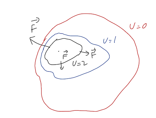
One more extremely useful observation: going back to the general case where \( \vec{\nabla} U \neq 0 \), we can see that if we take \( d\vec{r} \) in the direction perpendicular to \( \vec{\nabla} U \), then \( dU = 0 \). If we keep traveling in the direction perpendicular to \( \vec{\nabla} U \), we will trace out a line along which \( U \) is constant. This line is known as an equipotential. In fact, for a given \( \vec{\nabla} U \) there is a whole plane of perpendicular vectors we can choose, which means that in three dimensions we actually have a two-dimensional equipotential surface along which \( U \) doesn't change.
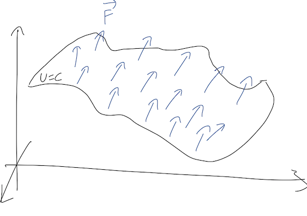
This gives us a useful way to visualize forces in two dimensions (the concept is still the same in three dimensions, but it's very hard to draw!) Consider a point particle moving in the \( (x,y) \) plane, subject to some unknown force. In two dimensions, equipotential surfaces will just be lines, so we can make a contour plot showing the lines of constant \( U \):
Some observations based on the plot:
- Notice that the equipotential lines never cross. This is basically true by definition: two different lines correspond to two different constant potential energies \( U_1 \) and \( U_2 \). Crossing would mean the potential can have two different values at the same point; our definition of a conservative force guarantees that can't be true.
- Since \( \vec{F} = - \vec{\nabla} U \), the force is in the direction perpendicular to the equipotential lines, as shown. The minus sign means that the direction of the force is "downhill", i.e. towards smaller values of \( U \).
- The spacing of the lines indicates how quickly \( U \) is changing vs. position, which means that a region which has lots of dense lines has a large gradient \( |\vec{\nabla} U| \), or equivalently, a large force \( |\vec{F}| \).
This plot may look familiar if you've ever read a topographic map, which shows lines of constant elevation in a top-down view:
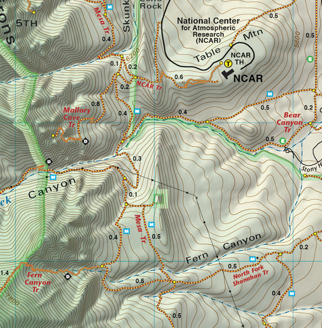
(source: https://www.latitude40maps.com/boulder-county-trails/)
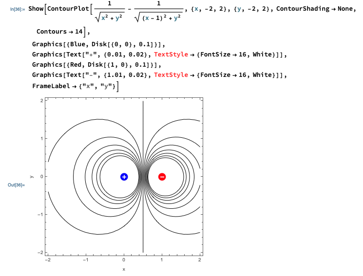
In fact, this is an equipotential contour plot for gravitational potential, since \( U(z) \propto z \)! (So in this case the "downhill" direction of the force vectors really is downhill!) This can give a useful metaphor for interpreting equipotential plots for other forces. Here's another example I've borrowed, showing equipotential contours for a pair of opposing electric charges:

(source: https://www.asc.ohio-state.edu/durkin.2/phys132/). This is not a plot of 3d equipotential surfaces: it's a two-dimensional plot (the bright lines are equipotential contours), with the third 'dimension' denoting the value of \( U(x,y) \).
Finally, you won't be surprised to learn that Mathematica has a function to make these plots for us, called ContourPlot[]. I won't dwell on the details, but here's a quick example showing how to make our own equipotential plot for a pair of electric charges.
Example: gradients and forces
As a quick example, suppose a particle has a potential energy function of the form
\[ \begin{aligned} U(x,y,z) = 3x \cos(y/L) - 2z^2 \end{aligned} \]
(ignoring units for now, this is a math exercise.) What is the force?
To find the force, we take the gradient: \( \vec{F} = -\vec{\nabla} U \). For the gradient, we need to know the partial derivatives of \( U \) with respect to all three coordinates. We haven't done any partial derivatives yet this semester, so let's go through them:
\[ \begin{aligned} \frac{\partial U}{\partial x} = 3 \cos (y/L) \\ \frac{\partial U}{\partial y} = -\frac{3x}{L} \sin (y/L) \\ \frac{\partial U}{\partial z} = -4z \end{aligned} \]
(finding partial derivatives is easy: we just ignore everything that we're not taking a derivative of.) Thus, the force is
\[ \begin{aligned} \vec{F} = -\vec{\nabla} U \\ = -\frac{\partial U}{\partial x} \hat{x} - \frac{\partial U}{\partial y} \hat{y} - \frac{\partial U}{\partial z} \hat{z} \\ = -3 \cos (y/L) \hat{x} + \frac{3x}{L} \sin (y/L) \hat{y} + 4z \hat{z}. \end{aligned} \]
Curl and Stokes' theorem
The operator \( \vec{\nabla} \) can be used to define other useful quantities, in addition to the gradient. One of these useful quantities is called the curl, where the curl of \( \vec{v} \) is denoted by \( \vec{\nabla} \times \vec{v} \). The cross product here is taken literally: the definition of curl is that we take the cross product of the gradient vector with the second vector. You'll remember that one way to write the cross product is using a 3x3 determinant; using this notation here, the curl is (in Cartesian coordinates)
\[ \begin{aligned} \nabla \times \vec{v} = \left|\begin{array}{ccc} \hat{x}&\hat{y}&\hat{z}\\ \frac{\partial}{\partial x}&\frac{\partial}{\partial y}&\frac{\partial}{\partial z}\\ v_x&v_y&v_z\end{array}\right| \\ = \left( \frac{\partial v_z}{\partial y} - \frac{\partial v_y}{\partial z} \right) \hat{x} + \left( \frac{\partial v_x}{\partial z} - \frac{\partial v_z}{\partial x} \right) \hat{y} + \left( \frac{\partial v_y}{\partial x} - \frac{\partial v_x}{\partial y} \right) \hat{z}. \end{aligned} \]
Now suppose we have a force \( \vec{F} \) which is conservative. By definition, that means we can find a potential function \( U \) so that \( \vec{F} = -\vec{\nabla} U \). But now notice what happens when we try to take the curl of \( \vec{F} \) and write it in terms of \( U \):
\[ \begin{aligned} (\vec{\nabla} \times \vec{F})_x = \frac{\partial F_z}{\partial y} - \frac{\partial F_y}{\partial z} \\ = \frac{\partial}{\partial y} \left( -\frac{\partial U}{\partial z} \right) - \frac{\partial}{\partial z} \left( -\frac{\partial U}{\partial y} \right). \end{aligned} \]
But the order of partial derivatives doesn't matter: there's only one \( \partial^2 U / \partial y \partial z \), so both terms are the same. Therefore, \( (\vec{\nabla} \times \vec{F})_x = 0 \). Of course, we didn't assume anything special about the \( x \)-direction, so it won't surprise you to know that the whole curl is in fact zero! We've just proved the vector identity
\[ \begin{aligned} \vec{\nabla} \times \vec{\nabla} U = 0 \end{aligned} \]
for any function \( U \). This means that if we have a conservative force, then its curl must be zero:
\[ \begin{aligned} \vec{\nabla} \times \vec{F} = 0. \end{aligned} \]
Curl looks like kind of a weird and arbitrary quantity, so you might wonder why we care if a force has zero curl or not. The short answer is that this identity goes both ways: if we're given a force \( \vec{F} \), we can calculate its curl, and if it is equal to zero then the force must be conservative. So curl allows us to test for a conservative force!
This is a big deal, because you'll remember that the second condition for a force to be conservative was that work done is independent of path, which is something you definitely can't test directly - there are always an infinite number of paths. But we argued that the path-independence of work is equivalent to the condition that
\[ \begin{aligned} \oint \vec{F} \cdot d\vec{r} = 0, \end{aligned} \]
i.e. the work vanishes on any closed path (a path that goes back to the same point, i.e. a loop.) But now we come to an important vector calculus result, Stokes' theorem, which I will state but not prove:
\[ \begin{aligned} \oint_{\partial \mathcal{S}} \vec{F} \cdot d\vec{r} = \int \hspace{-4mm} \int_{\mathcal{S}} (\vec{\nabla} \times \vec{F}) \cdot d\vec{A} \end{aligned} \]
Those are some pretty dense symbols, so in words: "Consider a finite surface \( \mathcal{S} \), with boundary curve \( \partial S \). The surface integral of the curl of any vector over \( \mathcal{S} \) is equal to the line integral of the same vector around the boundary \( \partial S \)."
We don't need to go too deep into surface integrals for our current purposes; as the name implies, they are the two-dimensional equivalent of a line integral. The important point right now is that if we have a force for which the curl \( \vec{\nabla} \times \vec{F} \) vanishes, then its line integral around any closed loop anywhere is automatically zero by Stokes' theorem. So there are several equivalent ways to state that a force \( \vec{F} \) is conservative:
- If the work done is path-independent;
- If \( \vec{F} = -\vec{\nabla} U \) for some function \( U \);
- If \( \vec{\nabla} \times \vec{F} = 0 \) everywhere.
Curl is much more important in electrodynamics; in mechanics, it's mostly important as a test for conservative forces. We'll have significantly more use for the divergence later on, but for now let's simply move on to our next topic.
Energy and one-dimensional systems
Although we've been working a lot in three dimensions with our vector calculus proofs, it turns out that some of the most powerful features of energy conservation arise in one-dimensional systems. It should be noted that "one-dimensional" here doesn't mean "only moving along a line"; it refers to any physical system in which we only need a single coordinate to tell us the full state of the system.
A basketball in freefall with no horizontal motion is a one-dimensional system (we just need the height \( y \)), but so is a pendulum (just need the angle \( \theta \)), or even a roller coaster (it's stuck on a track, so we can describe it in terms of \( s \), the distance along the track.) For simplicity, we'll call our single coordinate \( x \) in the following.
What about conservative forces? Taylor shows that because one-dimensional "paths" are very simple, any force which only depends on position is automatically conservative in one dimension. So as long as there's no dependence on other parameters like speed or time, any force in one dimension has a corresponding potential energy \( U(x) \), and
\[ \begin{aligned} F(x) = -\frac{dU}{dx}. \end{aligned} \]
In one dimension, equipotential surfaces aren't useful anymore - they would consist of some scattered points. Instead, we can visualize a problem by just plotting \( U(x) \) vs. \( x \). For example, here is the potential \( U(x) = \frac{1}{2} kx^2 \) corresponding to a mass on a spring, which is unstretched at \( x=0 \):
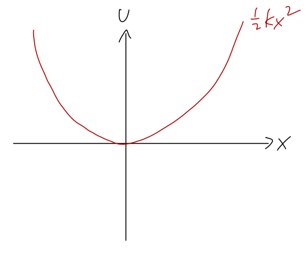
Again, the direction of the force is always "downhill", opposite the direction of increasing \( U \). We can also clearly see that there is an equilibrium point at \( x=0 \), where the potential is flat (\( dU/dx=0 \)) and therefore the force vanishes. (Equilibrium just means that the system will stay there if we start it there at rest.)
The potential carries a lot of useful information about a physical system, even in cases where we can't solve it completely! Once again, gravity will be a useful example and metaphor for understanding potentials in general. Imagine a roller coaster on a track. As a function of the distance \( x \) along the track, the height of the track \( y(x) \) will vary, usually in some complicated and interesting way. Since the gravitational potential is \( U(y) = +mgy \), that means that drawing the track is the same thing as drawing the potential energy!
Suppose we have a segment of roller coaster track that looks like this:
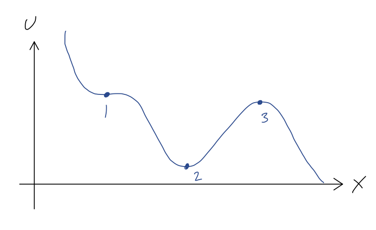
We can immediately see the points of equilibrium, marked 1, 2, and 3, where the force will vanish, and thus where the roller coaster cart would remain if it started at rest. We also get an immediate sense for the stability of these equilibria. A stable equilibrium point is one for which the system will remain near the equilibrium point if pushed slightly away; we can see that this is true at point 2, since if we give the cart a small push from this point, the force will always be directed back towards the lowest point.
An unstable equilibrium point is the opposite, a point where a small push will result in a large change in the system's position. This is clearly the case at point 3; for a small push away from point 3, the force points away from point 3, and the coaster will accelerate away - back towards point 2, or off to the right, depending on which way we push it.
Next time, we'll use Taylor series to make these statements more rigorous!