Last time, we were discussing equilibrium points (where \( dU/dx = 0 \)) in a one-dimensional roller coaster example:
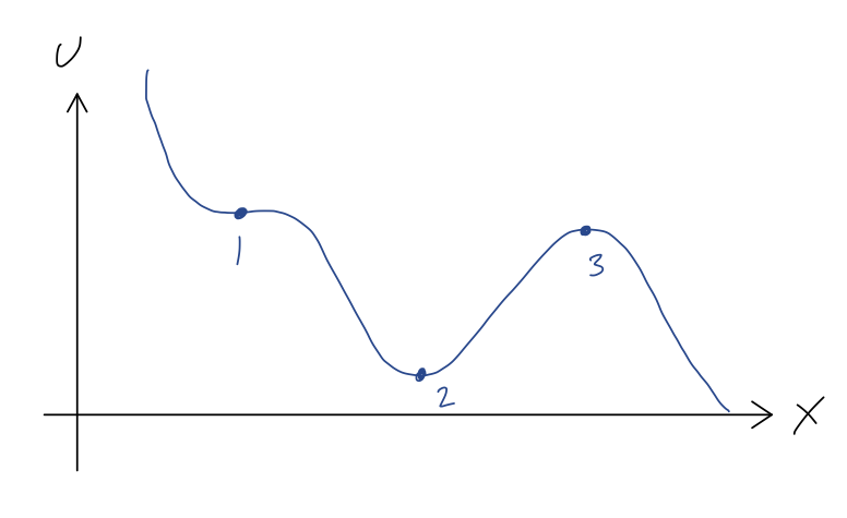
We can be more rigorous about these statements by consider a Taylor series expansion around each of these points. Let's start with point 2, and I'll use the shorthand notation \( U'(x) = dU/dx \) here. Since we already know that \( U'(x_2) = 0 \), the series expansion looks like
\[ \begin{aligned} U(x) \approx U(x_2) + \frac{1}{2} U''(x_2) (x-x_2)^2 + ... \end{aligned} \]
Now, we can't actually compute the second derivative, but we do know from the plot that it must be positive. (Our series expansion is telling us that \( U(x) \) looks like a parabola if we get close enough to \( x_2 \), and from the plot the parabola has to be opening upwards.) So if we define \( U''(x_2) = +k \) with \( k>0 \), then
\[ \begin{aligned} U(x) \approx U(x_2) + \frac{1}{2} k(x-x_2)^2 + ... \end{aligned} \]
near point 2. Taking the derivative of this series gives us the force,
\[ \begin{aligned} F(x) = -\frac{dU}{dx} = -k(x-x_2). \end{aligned} \]
This looks exactly like a spring force; it points towards \( x_2 \), no matter what value of \( x \) we use. We can go a step further and solve for the motion. Let's change coordinates so that \( u = x-x_2 \) is the distance to point 2. Then \( F(u) = -ku \), and the equation of motion is
\[ \begin{aligned} m\ddot{u} = -ku. \end{aligned} \]
We haven't considered general second-order ODEs yet, but we do know that this is a linear ODE, so it has a general solution containing 2 unknown constants, and we just need to find two different functions that go back to themselves with a minus sign after two derivatives. The basic trig functions both satisfy this property, so the solution is
\[ \begin{aligned} u(t) = A \cos (\sqrt{k/m} t) + B \sin (\sqrt{k/m} t). \end{aligned} \]
We don't need any more detail than this: the point is that since \( \sin \) and \( \cos \) both oscillate between \( -1 \) and \( +1 \), our total solution is bounded - it will always stay within some range of point 2.
If we expand around point 3, we find an almost identical story, except that now we find \( U''(x_3) = -\kappa \) with \( \kappa > 0 \), which gives us the equation of motion
\[ \begin{aligned} m\ddot{u} = +\kappa u \end{aligned} \]
now with \( u = x-x_3 \). Without the minus sign, the solutions we find are exponentials instead of trig functions:
\[ \begin{aligned} u(t) = Ae^{-\sqrt{\kappa/m} t} + Be^{+\sqrt{\kappa/m} t}. \end{aligned} \]
The second exponential term gets arbitrarily large as \( t \) gets bigger, so our solution is indeed unstable - it will run away from point \( x_3 \). Of course, the motion isn't exponential forever; we're doing a series expansion around \( x_3 \), so as soon as we get far enough away that the terms we dropped from the series become important, we can't use this simple solution for \( x(t) \) anymore.
Finally we come to point 1, which is sort of a tricky case; it is a saddle point of \( U(x) \), which means that the direction of the force depends on which way we push the cart. In physical terms, this is also an unstable equilibrium point. To see why, let's Taylor expand one more time. We still know that \( U'(x_1) = 0 \), but we must also have \( U''(x_1) = 0 \). (You may remember from calculus that this is the condition for a saddle point. More physically, if \( U''(x_1) \) wasn't zero, then close enough to \( x_1 \) our function would have to look parabolic, but that would mean it has to look like point 2 or point 3.) Thus, the series expansion here is
\[ \begin{aligned} U(x) \approx U(x_3) + \frac{1}{3!} U'''(x_3) (x-x_3)^3 + ... \end{aligned} \]
If we let \( U'''(x_3) = -q \) with \( q > 0 \) (convince yourself from the graph!), then the equation of motion is
\[ \begin{aligned} m\ddot{u} = \frac{1}{2} qu^2. \end{aligned} \]
We can't solve this analytically - there is no solution using elementary functions. But we don't need to, because it tells us what we need to know: the acceleration \( \ddot{u} \) is always positive, no matter the sign of \( u \) itself. So if we displace the cart from point 1 in either direction, it will be accelerated to the right - and since the acceleration increases as \( u \) increases, this solution is unstable and the cart moves away from point 1.
Equilibrium points are local statements about a physical system, but we can also say interesting and useful things about the global behavior using the one-dimensional potential. Since total energy \( E = T + U \) is conserved, if we know \( U(x) \) and the total energy, then we also know \( T(x) \). Instead of making a new plot, it's often useful to just draw the value of \( E \) as a dotted line on the plot for \( U(x) \).
For example, suppose the system begins at rest halfway between points 1 and 2. Then \( E = U(x_0) \), since at rest \( T=0 \). Let's draw it on the graph:
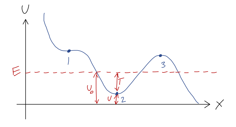
Since \( E = T + U \) and \( E \) is always the same, the difference between our dashed \( E \) line and the \( U(x) \) curve at any point is exactly the kinetic energy \( T \)! Now, since \( T = mv^2/2 \), it has the very important property that it can never be negative (note that \( U \) can be negative, and so can \( E \), because the value \( U=0 \) is arbitrary.) But that means that we can never have \( U > E \). So for the value of \( E \) shown, the cart can never reach point 1, point 3, or any part of the track above \( E \)!
This is a very simple but powerful observation: without knowing any of the details about how the cart moves with time, we know that its motion will never take it beyond the values of \( x \) where \( E = U(x) \). These points are called turning points, because if our object reaches one of them, it momentarily has \( T=0 \) and then turns around as the applied force pulls it back in the opposite direction.
The regions of the track where \( U > E \) are known as forbidden regions; we know the cart can never be found there. If all we know is \( E \), then the cart could be anywhere else; in this example, it could be in the potential well near point 2, or it could be on the downward-sloping track to the right of point 3. If we also know where the cart starts, then we can identify it as being stuck in one of these two regions, and it can never get to the other one. (Of course, as you know from modern physics, this is only true classically; a quantum roller coaster would be able to tunnel from one region to the other.)
Example: the pendulum, revisited
We've previously talked about the motion of a simple pendulum, and found the equation of motion awhile ago to be
\[ \begin{aligned} \ddot{\phi} = -\frac{g}{L} \sin \phi \end{aligned} \]
This is a non-linear differential equation, and there is no simple analytic solution to it at all. The usual procedure is to use the small-angle approximation, or numerical solution. But since this is a one-dimensional problem, we can instead write down the potential energy to make some useful observations!
Once again, here's a sketch of the pendulum setup:
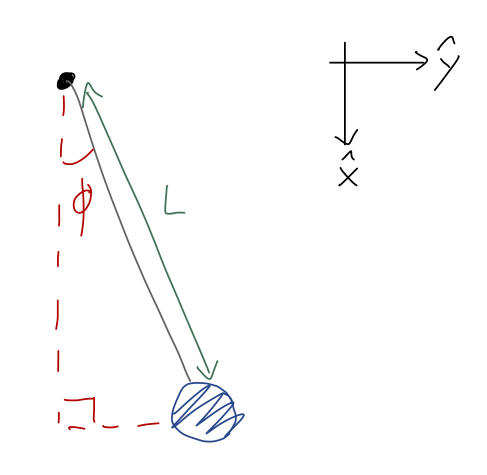
The only force acting is gravity, in the \( \hat{x} \) direction as the coordinates are drawn. Let's set the gravitational potential to be zero at the lowest point of the pendulum, when \( \phi = 0 \). With the origin at the pendulum support, we thus have
\[ \begin{aligned} U(x,y) = mg(L-x) = mgL(1 - \cos \phi) \end{aligned} \]
using \( x = L \cos \phi \). It's always a good idea to check that the sign makes sense here, so let's think about it: at \( \phi = 0 \), we have \( U = 0 \) as desired. At \( \phi = \pi/2 \), we have \( U = mgL \); the gravitational potential should be larger when the bob is higher, so this also checks out.
Let's sketch the potential as \( \phi \) changes from 0 to \( 2\pi \):
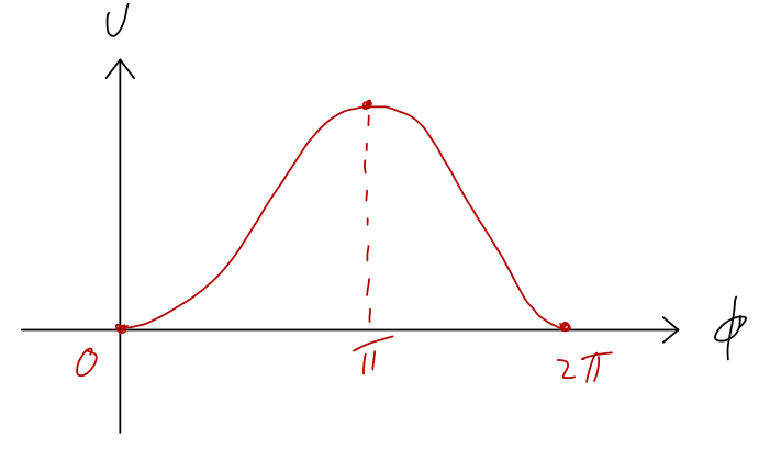
So we see two equilibrium points: in addition to the expected \( \phi = 0 \), there is also an unstable equilibrium at \( \phi = \pi \). This might seem a little weird, but if you think about it for a moment it makes intuitive sense: at exactly \( \phi = \pi \) the pendulum is perfectly balanced straight above the support.
Although it's easy to see graphically, let's exercise our Taylor series abilities to check the stability or instability of the two equilibrium points. To find equilibrium points in general, we solve for where the gradient of \( U \) vanishes, or:
\[ \begin{aligned} \frac{dU}{d\phi} = 0 = mgL \sin \phi \end{aligned} \]
which has solutions at \( \phi = 0, \pi, 2\pi, ... \), matching the points I already marked on the graph. Next, if we series expand the potential first at \( \phi = 0 \), we have
\[ \begin{aligned} U(\phi) \approx U(0) + \frac{1}{2} U''(0) \phi^2 + ... \\ = mgL(1 - \cos 0) + \frac{1}{2} (mgL \cos 0) \phi^2 + ... \\ = \frac{1}{2} mgL \phi^2 + ... \end{aligned} \]
which is indeed a stable equilibrium, since the coefficient of \( \phi^2 \) is positive. Note that I skipped the \( U' \) term in the expansion, since I already know it's zero at this point. Let's repeat the exercise at \( \phi = \pi \),
\[ \begin{aligned} U(\phi) \approx U(\pi) + \frac{1}{2} U''(\pi) (\phi-\pi)^2 + ... \\ = mgL(1 - \cos \pi) + \frac{1}{2} (mgL \cos \pi) (\phi-\pi)^2 + ... \\ = 2mgL - \frac{1}{2} mgL (\phi-\pi)^2 + ... \end{aligned} \]
which is indeed unstable: the potential looks like a downwards parabola near the point, and if we compute the force
\[ \begin{aligned} F(\phi) = -\frac{dU}{d\phi} = mgL(\phi - \pi) \end{aligned} \]
it will always point in the same direction as \( \phi \) if we move slightly away from the equilibrium, and we will be pushed away.
Moving beyond equilibrium, we can also use conservation of energy and turning points to say useful things about the motion, without having to assume a small angle. Suppose the pendulum starts at \( \phi = 0 \), and we give it a push so that it starts moving with initial speed \( v_0 \). What does its motion look like? The total energy is just \( T \) at \( \phi = 0 \), so we have
\[ \begin{aligned} E = T + U \\ \frac{1}{2} mv_0^2 = T + mgL(1 - \cos \phi) \end{aligned} \]
The turning points \( \phi_T \) occur where \( T = 0 \), or
\[ \begin{aligned} \frac{1}{2} mv_0^2 = mgL (1 - \cos \phi_T) \\ 1 - \cos \phi_T = \frac{v_0^2}{2gL} \\ \Rightarrow \cos \phi_T = \left( 1 - \frac{v_0^2}{2gL} \right). \end{aligned} \]
So although we don't know the detailed motion as a function of time, it's easy to find the maximum possible angle the pendulum will reach based on the initial speed. Notice that this works for any angle, but only for \( v_0^2 < 4gL \), at which point \( \phi_T = \pi \). For even larger initial speeds, there is no solution: we just have \( E > U \) everywhere, and the pendulum will just spin in a circle forever, in the absence of other forces.
If we really want to know about the motion as a function of time, there's one more nice trick we can do in one dimension. For any potential at all, the relation \( E = T + U \) in one dimension can be rewritten as:
\[ \begin{aligned} \frac{1}{2} m \dot{x}^2 = E - U(x). \end{aligned} \]
which we can solve for \( \dot{x} \):
\[ \begin{aligned} \dot{x} = \pm \sqrt{\frac{2}{m}} \sqrt{E - U(x)} \end{aligned} \]
(we would need extra information to figure out the sign, since \( T \) is the same for \( +\dot{x} \) and \( -\dot{x} \).) This is a first order and separable ODE - no matter how complicated \( U(x) \) is! So we can use it to write down a completely general solution: if \( x(0) = x_0 \), then
\[ \begin{aligned} t(x) = \pm \sqrt{\frac{m}{2}} \int_{x_0}^x \frac{dx'}{\sqrt{E-U(x')}} \end{aligned} \]
which we then have to invert to get \( x(t) \).
For the pendulum, this becomes
\[ \begin{aligned} t(\phi) = \pm \sqrt{\frac{m}{2}} \int_{\phi_0}^\phi \frac{d\phi'}{\sqrt{E - mgL(1 - \cos \phi')}} \end{aligned} \]
This is, unfortunately, one of those integrals that you can't actually do: it is used to define a special function called an elliptic function, which is the solution to the pendulum at all angles. So we didn't get something for nothing in this case. On the other hand, this can be a convenient way to do a numerical solution, since you don't need an ODE solver like Mathematica - you just need to do an integral.
Taylor explores a few other special topics in energy conservation, including the use of time-dependent potential energies (Taylor 4.5) and some more explorations of equilibrium and one-dimensional systems (4.7); I encourage you to read about these for your interest, but we won't go into them in any detail. Instead, we'll continue with his discussion of central forces, which will lead us into a detailed case study of the most important fundamental force in mechanics: gravity.