A central force is one for which in some choice of coordinates,
\[ \begin{aligned} \vec{F}(\vec{r}) = f(\vec{r}) \hat{r}. \end{aligned} \]
The concept is that the origin (i.e. the center of our coordinate system) is the source providing our central force, and the force at any point \( \vec{r} \) always points towards or away from this center. This should remind you a bit of drag forces, which we argued were always in the direction of \( \hat{v} \) (or opposite \( \hat{v} \), more precisely.) In both cases, we have a specific direction for the force by identifying where it comes from (motion for air resistance, and the source object for central force.)
A good example that you already know of a central force is just the electric force: if I put a charge \( Q \) at the origin, then the force on a second charge \( q \) sitting at point \( \vec{r} \) is
\[ \begin{aligned} \vec{F}_e(\vec{r}) = \frac{kqQ}{r^2} \hat{r}. \end{aligned} \]
As Taylor observes, this is a slightly more specialized version of a central force, because \( f(\vec{r}) = f(r) \), i.e. the magnitude of the force only depends on the distance between the charges. This is an example of spherical symmetry, or rotational invariance: in spherical coordinates, we can rotate our test charge \( q \) around in \( \theta \) and \( \phi \) as much as we want, and as long as \( r \) is held fixed the force magnitude is the same (although the direction changes so it's always pointing out from the origin.) As we'll prove in a moment, this is related to the question of whether or not we have a conservative central force. A static electric force is definitely conservative!
Gradient and curl in spherical coordinates
To study central forces, it will be easiest to set things up in spherical coordinates, which means we need to see how the curl and gradient change from Cartesian. Let's go through the derivation for the gradient - although this is something you can always look up, it's actually pretty easy, and the formula that you look up won't seem so arbitrary. Remember that in our derivation of gradient, we found the following infinitesmal relationship:
\[ \begin{aligned} dU = \vec{\nabla} U \cdot d\vec{r}. \end{aligned} \]
We have previously looked at how \( d\vec{r} \) changes if we switch coordinates: we can always start with the Cartesian version
\[ \begin{aligned} d\vec{r} = dx \hat{x} + dy \hat{y} + dz \hat{z} \end{aligned} \]
and just substitute in the change from \( (x,y,z) \) to \( (r,\theta,\phi) \). However, in this case it's probably easier to just start in spherical coordinates, where we know that simply \( \vec{r} = r \hat{r} \), and so taking the derivative with respect to some parameter \( s \),
\[ \begin{aligned} \frac{d\vec{r}}{ds} = \frac{dr}{ds} \hat{r} + r \frac{d\hat{r}}{ds}. \end{aligned} \]
Now we can relate the unit vector back to Cartesian coordinates:
\[ \begin{aligned} \hat{r} = \frac{1}{r} \left( x \hat{x} + y \hat{y} + z \hat{z} \right) \\ = \sin \theta \cos \phi \hat{x} + \sin \theta \sin \phi \hat{y} + \cos \theta \hat{z}. \end{aligned} \]
We can take a derivative with respect to \( s \) here, but it's better to remember that we eventually want our answer in terms of spherical unit vectors. Remember that we define the unit vectors as pointing in the direction of change with respect to a certain coordinate, so we can find them by looking at the derivatives of \( \hat{r} \):
\[ \begin{aligned} \frac{d\hat{r}}{d\theta} = \cos \theta \cos \phi \hat{x} + \cos \theta \sin \phi \hat{y} - \sin \theta \hat{z} \\ \frac{d\hat{r}}{d\phi} = - \sin \theta \sin \phi \hat{x} + \sin \theta \cos \phi \hat{y} \end{aligned} \]
and computing the lengths,
\[ \begin{aligned} \left| \frac{d\hat{r}}{d\theta} \right| = \cos^2 \theta (\cos^2 \phi + \sin^2 \phi) + \sin^2 \theta = 1 \\ \left| \frac{d\hat{r}}{d\phi} \right| = \sin^2 \theta (\sin^2 \phi + \cos^2 \phi) = \sin^2 \theta \end{aligned} \]
Now we use the chain rule:
\[ \begin{aligned} \frac{d\hat{r}}{ds} = \frac{d\hat{r}}{d\theta} \frac{d\theta}{ds} + \frac{d\hat{r}}{d\phi} \frac{d\phi}{ds} \\ = \left| \frac{d\hat{r}}{d\theta} \right| \hat{\theta} \frac{d\theta}{ds} + \left| \frac{d\hat{r}}{d\phi} \right| \hat{\phi} \frac{d\phi}{ds} \end{aligned} \]
on the last line using the definition of the unit vectors,
\[ \begin{aligned} \hat{\theta} = \frac{d\vec{r}/d\theta}{|d\vec{r}/d\theta|} = \frac{d\hat{r}/d\theta}{|d\hat{r}/d\theta|} \end{aligned} \]
where the second equality comes from the fact that the difference between \( \vec{r} \) and \( \hat{r} \) is a factor of the radius \( r \), which doesn't depend on the angle and so just cancels out. Combining our results above, we have
\[ \begin{aligned} \frac{d\hat{r}}{ds} = \frac{d\theta}{ds} \hat{\theta} + \sin \theta \frac{d\phi}{ds} \hat{\phi} \end{aligned} \]
or going all the way back to the start and cancelling out the \( ds \) infinitesmals,
\[ \begin{aligned} d\vec{r} = dr \hat{r} + r d\theta \hat{\theta} + r \sin \theta d\phi \hat{\phi}. \end{aligned} \]
This was a little bit of an algebra grind, but it's been a little while since we've done these sorts of coordinate manipulations so I thought the practice would be good! If you prefer a geometric derivation, Taylor does it that way without the algebra. In fact, it's pretty easy to see that this form makes sense from a little sketch:
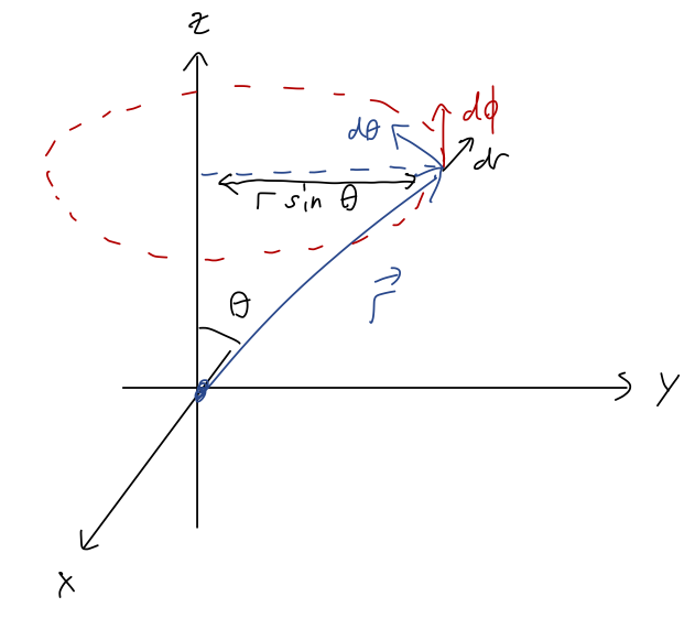
At fixed \( r \), in the \( \theta \) direction, we're always moving around a big circle of radius \( r \), so the infinitesmal arc length that we travel is \( ds = r d\theta \). In the \( \phi \) direction we're also tracing out a circle, but the size of that circle depends on \( \theta \), so \( ds = \rho d\phi = r \sin \theta d\phi \).
Back to the gradient! This was the hard part: to work out how the function \( U \) changes with respect to coordinates, we just apply the chain rule to find
\[ \begin{aligned} dU = \frac{\partial U}{\partial r} dr + \frac{\partial U}{\partial \theta} d\theta + \frac{\partial U}{\partial \phi} d\phi. \end{aligned} \]
No extra factors or coordinate changes to work about - since \( U \) is just a scalar function, the chain rule applies in this same simple way no matter what! Now we rewrite the original equation:
\[ \begin{aligned} dU = \vec{\nabla} U \cdot d\vec{r} \\ \frac{\partial U}{\partial r} dr + \frac{\partial U}{\partial \theta} d\theta + \frac{\partial U}{\partial \phi} d\phi = (\vec {\nabla} U) \cdot \left( dr \hat{r} + r d\theta \hat{\theta} +r \sin \theta d\phi \hat{\phi} \right) \end{aligned} \]
and just matching the \( dr, d\theta, d\phi \) terms on both sides, we find
\[ \begin{aligned} \vec{\nabla} U = \frac{\partial U}{\partial r} \hat{r} + \frac{1}{r} \frac{\partial U}{\partial \theta} \hat{\theta} + \frac{1}{r \sin \theta} \frac{\partial U}{\partial \phi} \hat{\phi}. \end{aligned} \]
The bad news is that we actually can't simply derive the curl or divergence from the gradient in spherical or cylindrical coordinates. This is basically for the same reason that Newton's laws become more complicated in these coordinate systems: the unit vectors themselves become coordinate-dependent, so extra terms start to pop up related to derivatives acting on unit vectors.
The correct way to derive the curl in spherical coordinates would be to start with the Cartesian version and carefully substitute in our coordinate changes for the unit vectors and for \( (x,y,z) \rightarrow (r,\theta,\phi) \). This is straightforward but tedious, so I'll skip to the result: the curl in spherical coordinates takes the form, in determinant notation,
\[ \begin{aligned} \vec{\nabla} \times \vec{A} = \frac{1}{r^2 \sin \theta} \left| \begin{array}{ccc} \hat{r} & r \hat{\theta} & r \sin \theta \hat{\phi} \\ \frac{\partial}{\partial r} & \frac{\partial}{\partial \theta} & \frac{\partial}{\partial \phi} \\ A_r & r A_\theta & r \sin \theta A_\phi \end{array} \right| \end{aligned} \]
Let's use this to compute the curl of central force vector \( \vec{F}(\vec{r}) = f(\vec{r}) \hat{r} \) in spherical coordinates:
\[ \begin{aligned} \vec{\nabla} \times \vec{F}(\vec{r}) = \frac{1}{r^2 \sin \theta} \left| \begin{array}{ccc} \hat{r} & r\hat{\theta} & r\sin \theta \hat{\phi} \\ \frac{\partial}{\partial r} & \frac{\partial}{\partial \theta} &\frac{\partial}{\partial \phi} \\ f(\vec{r}) & 0 & 0 \end{array} \right| \\ = \frac{1}{r \sin \theta} \frac{\partial f}{\partial \phi} \hat{\theta} - \frac{1}{r} \frac{\partial f}{\partial \theta} \hat{\phi}. \end{aligned} \]
So we can see right away that the condition for the curl to vanish - and therefore for \( \vec{F}(\vec{r}) \) to be conservative - is that both \( \partial f/\partial \phi \) and \( \partial f/\partial \theta \) should be zero, or in other words the magnitude should only depend on the radius,
\[ \begin{aligned} f(\vec{r}) = f(r). \end{aligned} \]
You can also prove this by using the gradient and matching on to the fact that \( \vec{F} \) has to point in the \( \hat{r} \) direction; convince yourself from the formula for \( \vec{\nabla} U \) we found, or read the argument in Taylor.
Two-particle central forces
Conservative central forces are common in physics, particularly for fundamental forces: both electric force and gravitational force are central and conservative. One of the really nice features of such a force is that since the magnitude only depends on \( r \), the distance to the source, many aspects of their physics can be treated as one-dimensional; we've already seen how that can be a really powerful simplification.
However, this setup so far forces a coordinate choice on us: we have to put our source at the origin. But what if we have two particles that are both sources, and are both moving - how can we describe their effects on each other through a central force? More generally, what if we have an extended source which is larger than a point - where do we put the origin?
We'll start by generalizing to the two-particle case, which will be the hard part; taking the next step to extended sources will be easy. We start with two particles labelled \( 1 \) and \( 2 \), at positions \( \vec{r}_1 \) and \( \vec{r}_2 \) like this:
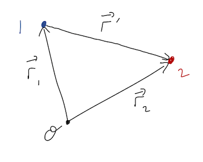
No external forces are present, but as shown, we assume that the particles are exerting a central force on one another. Defining the \( \hat{r}' \) vector pointing from 1 to 2 as shown, we have from the definition of a central force
\[ \begin{aligned} \vec{F}_{12} = f(\vec{r}') \hat{r}' \\ \vec{F}_{21} = -f(\vec{r}') \hat{r}' \end{aligned} \]
where we notice that Newton's third law requires the magnitude to be the same function, so that these are equal and opposite. Now, \( \vec{r}' \) isn't some unknown, it's related to the positions of our two objects:
\[ \begin{aligned} \vec{r}' = \vec{r}_1 - \vec{r}_2 \end{aligned} \]
(easier to see in the form \( \vec{r}_1 + \vec{r}' = \vec{r}_2 \)), and for the corresponding unit vector
\[ \begin{aligned} \hat{r}' = \frac{\vec{r}'}{|\vec{r}'|} = \frac{\vec{r}_1 - \vec{r}_2}{|\vec{r}_1 - \vec{r}_2|}. \end{aligned} \]
Since the central force only acts in the \( \vec{r}' \) direction, the point is that we can just solve for the relative motion of our two objects, and we're back to having just one vector to worry about instead of two. So we don't have to push one object to the origin for a central force to be a useful description of two objects - we just focus on their relative position.
You might object that just knowing the relative position isn't enough information! We have two particles, which means we need 6 numbers to describe where they both are at any given moment, but \( \vec{r}' \) only has three components. In fact, we can get the other three components using the center of mass: because we've specified no external forces, we have for the CM position
\[ \begin{aligned} M \ddot{\vec{R}} = \vec{F}_{\rm ext} = 0 \end{aligned} \]
which gives us the other three equations we need to fully keep track of everything.
What if we have not just a central force, but a conservative force? We know that \( f(\vec{r}') \) becomes just \( f(r') \) - that is, the force will only depend on the distance between our two particles and nothing else. As a result, we can write a single potential energy function \( U(r') \) that will describe the force \( f(\vec{r}') \). To get the individual forces from the potential, we take gradients with respect to each coordinate:
\[ \begin{aligned} \vec{F}_{12} = -\vec{\nabla}_1 U(r') \\ \vec{F}_{21} = -\vec{\nabla}_2 U(r') \end{aligned} \]
where the subscript gradient means "take derivatives with respect to the given coordinate", for example in Cartesian coordinates
\[ \begin{aligned} \vec{\nabla}_1 = \frac{\partial}{\partial x_1} \hat{x}_1 + \frac{\partial}{\partial y_1} \hat{y}_1 + \frac{\partial}{\partial z_1} \hat{z}_1 \end{aligned} \]
ignoring the coordinates of \( \vec{r}_2 \). It's easy to show from the definition of \( \vec{r}' \) that this definition gives us equal and opposite forces as required by the third law (try it yourself!)
Taylor has a very thorough discussion of how all of this generalizes beyond two particles, to the general \( N \)-particle case: the punchline is that we can always define a combined potential energy \( U \) for all our particles, the force on any given particle is
\[ \begin{aligned} \vec{F}_\alpha = -\vec{\nabla}_\alpha U(\vec{r}_1, \vec{r}_2, ..., \vec{r}_N) \end{aligned} \]
and the total energy \( E = T_1 + T_2 + ... + T_N + U \) is always conserved (if the forces involved are conservative - which we've sort of assumed by writing a \( U \) in the first place, but there are some edge cases like time-dependent potential energies that Taylor talks about.)
I will just let you read the Taylor derivation and not go over it here; it's an important fundamental result, but it doesn't really show off any math that we haven't seen before, and it's not something we'll need to work with practically. Instead, let's move on to consider a single conservative, central force in detail: gravity!
Gravitational force
Our starting point is Newton's general law of gravitation. If we have a source mass \( M \) at the origin, and a test mass \( m \) at \( \vec{r} \), the force of gravity acting on the test mass is
\[ \begin{aligned} \vec{F}_g = -\frac{GMm}{r^2} \hat{r}. \end{aligned} \]
The "gravitational charge" of an object is just its mass. Since mass is always positive, the force of gravity is always attractive - it pulls the two objects together, or in this case, pulls the mass \( m \) towards the origin. The constant \( G \) is known as the gravitational constant, Newton's constant or just "big G"; its best value, according to NIST CODATA, is
\[ \begin{aligned} G = 6.67430(15) \times 10^{-11}\ {\rm m}^3 / {\rm kg} / {\rm s}^2. \end{aligned} \]
The corresponding potential energy function is
\[ \begin{aligned} U(r) = -\frac{GMm}{r} \end{aligned} \]
(note that this is also negative, since the gradient gives us an extra minus sign.) We can add an arbitrary constant to it; the choice above with no constant corresponds to choosing our zero point at infinity, i.e. \( \lim_{r \rightarrow \infty} U(r) = 0 \). You can also remember the sign on physical grounds: it takes work to push two massive objects apart against gravity, so \( U \) should increase as \( r \) increases, which it does with the minus sign.
The gravitational force closely resembles the electric force, and in a similar way to the electric example, we can define a gravitational field \( \vec{g} \) by dividing out the "charge" (the mass in this case), such that
\[ \begin{aligned} \vec{F}_g = m\vec{g}. \end{aligned} \]
From above, the gravitational field generated by a point mass \( M \) is then
\[ \begin{aligned} \vec{g} = -\frac{GM}{r^2} \hat{r}. \end{aligned} \]
There isn't a whole lot of interesting physics we can do with just two masses, as it turns out. So what happens if we have multiple sources? Since multiple forces acting on a simple object just add together, we can also add together the gravitational fields from multiple sources to get a single, combined field:
\[ \begin{aligned} \vec{g} = \vec{g}_1 + \vec{g}_2 + ... = -\frac{GM_1}{r_1^2} \hat{r}_1 -\frac{GM_2}{r_2^2} \hat{r}_2 + ... \end{aligned} \]
This is the starting point we need to talk about extended sources, which will let us do some realistic applications of gravity, such as the Earth's gravitational field.