To deal with realistic objects, we'd like to be able to calculate the gravitational field due to a continuous object with some density. Recalling our previous example of finding the center of mass, we can think of this as just adding up all of the contributions from infinitesmal bits of mass \( dm \) inside of an object. For the center of mass, recall we had
\[ \begin{aligned} M = \sum_\alpha m_\alpha,\ \ \vec{R} = \frac{1}{M} \sum_\alpha m_\alpha \vec{r}_\alpha \end{aligned} \]
which became for continuous objects
\[ \begin{aligned} M = \int dm = \int \rho(\vec{r}) dV,\\ \vec{R} = \frac{1}{M} \int \vec{r} dm = \frac{1}{M} \int \vec{r} \rho(\vec{r}) dV. \end{aligned} \]
Similarly, for an extended massive source, we can add up all of the contributions to the gravitational field from individual pieces. However, this is going to be a little more complicated, so we should start with a diagram:

As pictured, we have to keep track of the location \( \vec{r}' \) of our source mass, but also the position \( \vec{r} \) where we want to know the field. As a sum over individual masses \( m_\alpha \), we have
\[ \begin{aligned} \vec{g} = \sum_\alpha -\frac{Gm_\alpha}{|\vec{s}_\alpha|^2} \hat{s}_\alpha \end{aligned} \]
where \( \vec{s} = \vec{r} - \vec{r}'_\alpha \) is the vector pointing from the source mass \( \alpha \) to the position \( \vec{r} \). (Some books will refer to this using a funny-looking script \( r \); I think this is confusing, and I also don't know how to typeset the weird \( r \), so I'll use \( s \).)
We find the continuous version by replacing \( m \) with the density \( \rho \):
\[ \begin{aligned} \vec{g} = -G \int \frac{dm}{|\vec{s}|^2} \hat{s} \\ = -G \int \frac{dV' \rho(\vec{r}')}{|\vec{r} - \vec{r}'|^3} (\vec{r} - \vec{r}') \end{aligned} \]
where I've written out \( \hat{s} \) in terms of the other vectors, which gives us an extra factor of \( 1/|\vec{s}| \). As the prime on \( dV' \) indicates, we're integrating over all possible positions \( \vec{r'} \) of the source mass \( dm \). We can do a \( u \)-substitution to think of the integral as being over the relative position vector \( \vec{s} \), but that hides the dependence on \( \vec{r} \) which is important to keep in mind.
This looks pretty horrible compared to the center of mass integral! Much of the complication comes from the fact that we have a second vector \( \vec{r} \) in addition to the one that we're trying to integrate over. We'll do a couple of examples, but I'll emphasize from the start that it is very important to make sketches and think carefully about these vectors when trying to calculate \( \vec{g} \)!
Symmetry will also be very useful, as with the center of mass. In particular, suppose we are at the origin and there are two equal pieces of mass at \( +\vec{s} \) and \( -\vec{s} \), exactly on opposite sides:
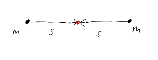
Then the total gravitational field is
\[ \begin{aligned} \vec{g} = -\frac{Gm}{s^2} \hat{s} - \frac{Gm}{s^2} (-\hat{s}) = 0. \end{aligned} \]
In other words, just as we saw for the CM position, the contributions of two equal masses at opposite positions to the \( \vec{g} \) field cancel exactly. This reflection-symmetry observation will extend to a whole object: if we have two solid hemispheres with the same mass and shape, then at the point exactly in between their centers, \( \vec{g} = 0 \) without having to calculate anything.
This can also work component by component. If we have our two equal masses at \( (+x',0,0) \) and \( (-x',0,0) \), and we're interested in the gravitational field along the \( y \) axis:
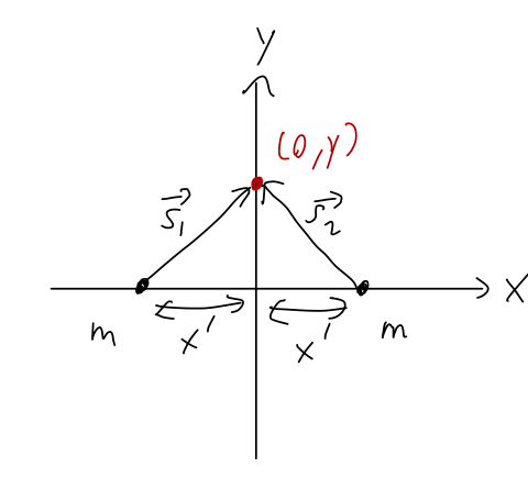
then we have
\[ \begin{aligned} \vec{g} = -\frac{Gm}{(x^2 + y^2)^{3/2}} (x\hat{x} + y \hat{y}) - \frac{Gm}{(x^2 + y^2)^{3/2}} (-x \hat{x} + y \hat{y}) \end{aligned} \]
writing out the unit vectors in our \( x,y \) coordinates. So in the \( x \)-direction, we have an exact cancellation again, and \( g_x = 0 \). However, we still have a contribution in the \( y \)-direction:
\[ \begin{aligned} \vec{g} = -\frac{2Gmy}{(x^2 + y^2)^{3/2}} \hat{y}. \end{aligned} \]
This will give us a messy equation of motion, thanks to the \( 3/2 \) power in the denominator! But we can at least see that the force is always attractive towards \( y=0 \), as we might guess, so if we release a point particle somewhere on the \( y \)-axis, we would expect it to just oscillate back and forth along the \( y \)-axis. (In fact, this is a perfect case for a one-dimensional potential analysis!)
Example: gravitational field of a disk
Let's try a more interesting example of finding \( \vec{g} \) to see how this works in practice with an extended object, instead of just point masses. Suppose we have a solid but very thin disk of constant area mass density \( \sigma \) (units: kg/\( {\rm m}^2 \)) and radius \( R \).
To deal with a thin disk, our integral over \( dV \) will become just a two-dimensional area integral \( dA \), since the \( z \)-direction is infinitesmally thin. (If you're not happy with this hand-waving approximation, you can calculate the three-dimensional version of this for a height \( h \), and then take the limit \( h \rightarrow 0 \). You should get the same results we're about to find.)
Now, as with the center of mass, we can view the equation for \( \vec{g} \) as just three separate integrals to do for each of the components \( g_x, g_y, g_z \). In general, we need to calculate all three of them, but symmetry can save us by telling us certain components are automatically zero. However, things are complicated by the fact that we have to choose the point \( \vec{r} \) to calculate the field at. For a completely arbitrary point in space, symmetry won't help us for the disk!
But let's say we want to calculate the field directly above the center of the disk, along the \( z \)-axis:
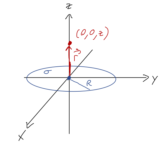
Then we have \( \vec{g}_x = \vec{g}_y = 0 \) thanks to reflection symmetry (remember, it's the reflection of the relative \( \vec{s} \) vector that matters, which is why we had to specify \( \vec{r} = z\hat{z} \) first!) Let's convince ourselves by actually setting up one of the integrals:
\[ \begin{aligned} g_x = -G \int \frac{dA' \sigma}{|\vec{r} - \vec{r}'|^3} (\vec{r} - \vec{r}')_x \\ = G \sigma \int \frac{dA' x'}{(x'^2 + y'^2 + z^2)^{3/2}} \end{aligned} \]
using \( \vec{r} - \vec{r}' = -x' \hat{x} - y' \hat{y} + z \hat{z} \), from the diagram. Now, this is already good enough to see the cancellation: because the integrand has a single \( x' \) upstairs, for every point on the disk at \( (+x', +y') \) there will be an equal and opposite contribution from \( (-x',y') \), so the whole thing will be zero. To see it even more explicitly, we should really change to cylindrical coordinates \( (\rho', \phi') \) inside the integral:
\[ \begin{aligned} g_x = G \sigma \int_0^{2\pi} d\phi' \int_0^R d\rho' \frac{\rho'^2 \cos \phi'}{(\rho'^2 + z^2)^{3/2}} \end{aligned} \]
The \( \phi' \) integral is the one that matters, and it's easy to do: we have
\[ \begin{aligned} \int_0^{2\pi} d\phi' \cos \phi' = \left. \sin \phi'\right|_0^{2\pi} = 0. \end{aligned} \]
Since the choice of \( x \)-direction vs. \( y \)-direction on a disk is totally arbitrary, clearly the same setup will give us \( g_y = 0 \) as well. Now let's move on to the non-zero part of the field, \( g_z \). Since we've already gone through the details of the setup for \( x \), it should be easy to see that
\[ \begin{aligned} g_z = -G \sigma \int_0^{2\pi} d\phi' \int_0^R d\rho' \frac{\rho' z}{(\rho'^2 + z^2)^{3/2}} \\ = -2\pi G \sigma z \int_0^R \frac{d\rho' \rho'}{(\rho'^2 + z^2)^{3/2}}. \end{aligned} \]
This is actually a very friendly integral for \( u \)-substitution! Let's pick \( u = \rho'^2 + z^2 \), which gives \( du = 2\rho' d\rho' \). Then
\[ \begin{aligned} g_z = -2\pi G \sigma z \int_{z^2}^{R^2 + z^2} \frac{du/2}{u^{3/2}} \\ = -\pi G \sigma z \left( \left. -\frac{2}{u^{1/2}} \right|_{z^2}^{R^2+z^2} \right) \\ = 2\pi G \sigma z \left( \frac{1}{\sqrt{R^2 + z^2}} - \frac{1}{|z|} \right). \\ \end{aligned} \]
We could replace the density \( \sigma \) with the total mass \( M \); since it's a two-dimensional density, we have \( M = \sigma \pi R^2 \). But there's no normalizing \( 1/M \) like there is for the center of mass, so for this calculation it's fine to just leave it in terms of \( \sigma \) in general.
Let's do some basic sanity checks! First of all, the sign: since \( \sqrt{R^2 + z^2} > |z| \) always, we have (1/big - 1/small) so the whole field is proportional to \( -z \). This makes sense - the direction of the field, and thus of the gravitational force \( \vec{F} = m\vec{g} \) on a test mass, always points towards the disk at \( z=0 \).
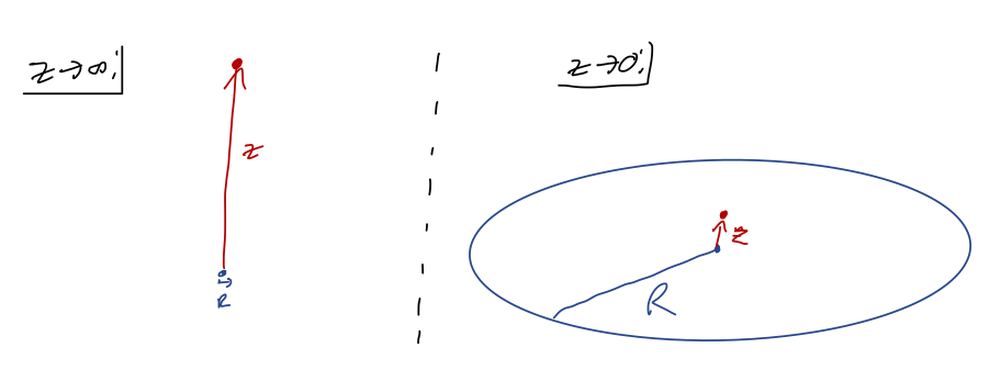
What about the limits? As \( z \rightarrow 0 \), approaching the disk, we have
\[ \begin{aligned} g_z \rightarrow 2\pi G \sigma z \left( \frac{1}{R} - \frac{1}{|z|} \right) \approx -2\pi G \sigma \frac{z}{|z|} \end{aligned} \]
which is a constant - the fraction \( z/|z| \) just gives us either +1 above the disk or -1 below it, ensuring that the field points towards the disk. This makes sense: if we get arbitrarily close to the disk, from our perspective it will look just like standing on a very large flat surface, from which we would expect just a constant gravity field pointing "down".
The other limit to consider is \( z \rightarrow \infty \). This means that \( z \gg R \), which we can use to series expand the first term in the field:
\[ \begin{aligned} \frac{1}{\sqrt{R^2 + z^2}} = \frac{1}{|z|} \frac{1}{\sqrt{1 + (R/z)^2}} \end{aligned} \]
Let's use the binomial formula to expand,
\[ \begin{aligned} (1+z)^n = 1 + nz + \frac{n(n-1)}{2} z^2 + ... \end{aligned} \]
which leads to, just keeping the first two terms,
\[ \begin{aligned} \frac{1}{\sqrt{R^2 + z^2}} \approx \frac{1}{|z|} \left(1 - \frac{R^2}{2z^2} + ... \right) \end{aligned} \]
The \( 1/|z| \) terms cancel off, and we're left with
\[ \begin{aligned} g_z \rightarrow 2\pi G \sigma \frac{z}{|z|} \left( -\frac{R^2}{2z^2} + ... \right) \end{aligned} \]
Now it's useful to substitute in \( M = \pi R^2 \sigma \), which will absorb the \( R^2 \) factor and leave us with
\[ \begin{aligned} g_z \rightarrow -\frac{GM}{z^2} \frac{z}{|z|} \end{aligned} \]
or \( \vec{g} = -GM/z^2 \hat{r} \), along the \( z \)-axis. So in this limit, the leading dependence on \( R \) vanishes and we just recover the single point-particle form of the gravitational field! This makes a lot of sense: if we're really, really far away from the disk, then the fact that it's an extended object doesn't really matter - in fact, from far enough away we probably wouldn't be able to tell that it has any radius, we would just see a point.
Gravitational potential of extended objects
So far, we haven't really used the fact that gravity is a conservative force. In fact, being able to write a potential energy function \( U(\vec{r}) \) can actually save us a lot of work when dealing with extended objects! Recall that the potential energy for a single test mass \( m \) in the gravity field of a source mass \( M \) is
\[ \begin{aligned} U(r) = -\frac{GMm}{r}. \end{aligned} \]
What if we have multiple sources? I'll skip the detailed derivation, but the answer is that we can simply add the potential energies: for example, in the following situation
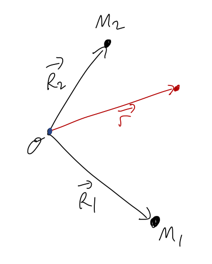
we just have
\[ \begin{aligned} U(\vec{r}) = -\frac{GM_1 m}{|\vec{r} - \vec{R}_1|} - \frac{GM_2 m}{|\vec{r} - \vec{R}_2|}. \end{aligned} \]
It's straightforward to see that taking \( \vec{F}_g = -\vec{\nabla} U \), where \( \vec{\nabla} \) is the gradient with respect to the \( \vec{r} \) coordinates, adding the potentials like this is equivalent to adding the gravitational forces together.
One more definition before we continue: like the force, the potential energy depends on the test mass \( m \), but in a very trivial way. It's often useful to factor out the \( m \) so we can calculate a function that only depends on the sources, which we can then apply to any test mass (or collection of test masses.) So just like we defined \( \vec{F}_g = m\vec{g} \), we now define the gravitational potential for a point source to be
\[ \begin{aligned} \Phi(r) = -\frac{GM}{r} \end{aligned} \]
so that \( U(r) = m\Phi(r) \). We can immediately see that \( \vec{g} = -\vec{\nabla} \Phi \), so this gives us another way to find the gravitational field. Potential is an unfortunate name for this quantity - keep in mind that \( \Phi \) is not a potential energy, it has the wrong units! This is completely analogous to the electric potential \( V(r) \), which is also not a potential energy - but the combination \( qV \) is.
Now if we have an extended object, as we saw before:
then the potential at position \( \vec{r} \) due to the infinitesmal source \( dm \) is
\[ \begin{aligned} d\Phi(\vec{r}) = -\frac{G dm}{s} = -\frac{G dm}{|\vec{r}' - \vec{r}|}, \end{aligned} \]
and thus the total potential is
\[ \begin{aligned} \Phi(\vec{r}) = -G \int \frac{dV' \rho(\vec{r}')}{|\vec{r}' - \vec{r}|}. \end{aligned} \]
This is much nicer to evaluate than the integrals we had to do for \( \vec{g} \)! Now we have no vector components to worry about - just a single scalar quantity. We can then take the gradient of our result (with respect to \( \vec{r} \)) to find the gravitational field \( \vec{g} \).
Next time: an example of calculating the potential for an extended object.