Last time, we started talking about Gauss's law, which through the divergence theorem is equivalent to the relationship
\[ \begin{aligned} \vec{\nabla} \cdot \vec{g} = -4\pi G \rho(\vec{r}). \end{aligned} \]
This equation is sometimes also called Gauss's law, because one version implies the other one thanks to the divergence theorem. This last equation is also interesting, because we can view it as a differential equation that can be solved for \( \vec{g} \) given \( \rho(\vec{r}) \) - yet another way to obtain the gravitational vector field!
Actually, there's one more simplification we can make here. Remember that the gravitational field is related to the potential as \( \vec{g} = -\vec{\nabla} \Phi \). If we plug this in, we find the equation
\[ \begin{aligned} \nabla^2 \Phi(\vec{r}) = 4\pi G \rho(\vec{r}), \end{aligned} \]
where \( \nabla^2 \) is another new operator called the Laplacian, which is basically the dot product of the gradient \( \vec{\nabla} \) with itself. In Cartesian coordinates,
\[ \begin{aligned} \nabla^2 \Phi = \frac{\partial^2 \Phi}{\partial x^2} + \frac{\partial^2 \Phi}{\partial y^2} + \frac{\partial^2 \Phi}{\partial z^2}. \end{aligned} \]
This differential equation relating \( \Phi \) directly to \( \rho \) is known as Poisson's equation. For some applications, it's the most convenient way to solve for the gravitational field, since we don't have to worry about vectors at all: we get the scalar potential from the scalar density. In particular, Poisson's equation is often a useful way to solve numerically for the potential due to a complicated source density.
We won't use the differential versions of these equations in practice this semester, but they are very useful for more than just numerical solutions: you'll probably see a lot of them when you take electricity and magnetism. But I wanted to explain in a bit more detail where Gauss's law comes from.
Having covered the math, I should say a little bit more about the physical interpretation of Gauss's law. The quantity on the left-hand side, \( \oint_{\partial V} \vec{g} \cdot d\vec{A} \), is known as the gravitational flux through the surface \( \partial V \). There are some hand-waving arguments people sometimes like to make about "counting field lines" to think about flux, but obviously this is a little inaccurate since the strength \( |\vec{g}| \) of the field matters and not just the geometry. Still, a physical way to state Gauss's law is: "for a surface with no enclosed mass, the net gravitational flux through the surface is zero."
Example: gravity far from an arbitrary source
Now let's see the practical use of the integral form of Gauss's law that we wrote down above. I'll use it to prove a very general result that was hinted at by our solutions above: for any massive object of size \( R \), the gravitational field at distances \( r \gg R \) will be exactly the field of a point mass and nothing more. Let's draw a spherical surface of size \( r \gg R \) around our arbitrary object of mass \( M \):
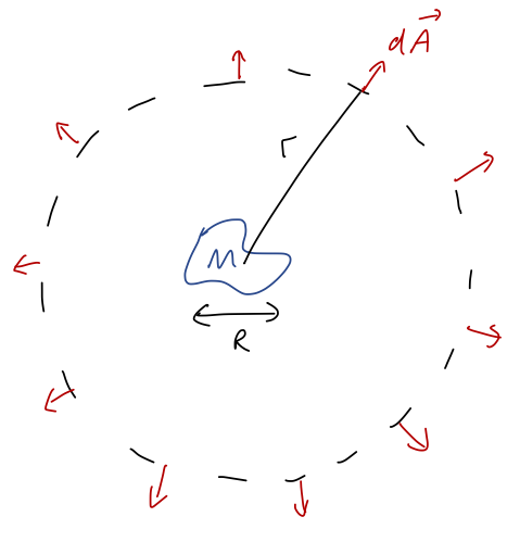
The spherical surface we've chosen here is known as a Gaussian surface - it defines the vector \( d\vec{A} \) and is crucial in applying Gauss's law. We always want to choose the Gaussian surface to match the symmetries of our problem. Since we don't know what \( \vec{g}(\vec{r}) \) is yet, our objective is to choose the right simplifications so we can pull \( \vec{g} \) out of the integral on the left-hand side.
Since \( r \) is much larger than \( R \), the volume integral on the right-hand side of Gauss's law always includes the entire object, and we just get the total mass \( M \). So in other words, for any choice of \( r > R \), we have
\[ \begin{aligned} \oint_{\partial V} \vec{g}(\vec{r}) \cdot d\vec{A} = -4\pi G M. \end{aligned} \]
With our choice of a spherical surface as \( \partial V \), the vector \( d\vec{A} \) is always in the \( \hat{r} \) direction. Explicitly in spherical coordinates,
\[ \begin{aligned} \int_0^{2\pi} d\phi \int_0^\pi d\theta (r^2 \sin \theta) \vec{g}(\vec{r}) \cdot \hat{r} = -4\pi G M \end{aligned} \]
Now let's think about the field \( \vec{g}(\vec{r}) \). If our object were perfectly symmetric, like a sphere, then any components not in the radial direction would cancel off as we've seen, and we would have \( \vec{g}(\vec{r}) = g(r) \hat{r} \). On the other hand, what if it wasn't perfectly symmetric? That would mean we have an imperfect cancellation between the field contributions from two bits of mass that are no more than \( R \) apart from each other. But the contribution from two such pieces has to be something like
\[ \begin{aligned} |\Delta g(\vec{r})| \sim \frac{1}{|\vec{r}'_1 - \vec{r}|^2} - \frac{1}{|\vec{r}'_2 - \vec{r}|^2} \\ = \frac{1}{r^2} \left(1 + \frac{2|\vec{r}'_1|}{r} + ... \right) - \frac{1}{r^2} \left(1 + \frac{2|\vec{r}'_2|}{r} + ... \right) \end{aligned} \]
The \( 1/r^2 \) parts cancel off nicely, so the leading term is something like \( (|\vec{r}'_1| - |\vec{r}'_2|) / r^3 \). But this can't be any larger than \( R/r^3 \), which is \( R/r \) smaller than the leading \( 1/r^2 \) term. In other words, we know that
\[ \begin{aligned} \vec{g}(\vec{r}) = g(r) \hat{r} + \mathcal{O} \left(\frac{R}{r} \right) \end{aligned} \]
even if our object isn't spherically symmetric. If we only keep the leading term, then the integral simplifies drastically:
\[ \begin{aligned} -4\pi G M = \int_0^{2\pi} d\phi \int_0^\pi d\theta \sin \theta r^2 g(r) = 4\pi r^2 g(r) \end{aligned} \]
and since there's no \( r \)-integral, we just have
\[ \begin{aligned} g(r) = -\frac{GM}{r^2} \end{aligned} \]
up to corrections of order \( R/r \), as I assumed.
This is a nice confirmation of the arguments I made above, that everything looks like a point mass if you're far enough away! It's also a simple example of how we use Gauss's law in practice: it's most useful if some symmetry principle lets us identify the direction of \( g(r) \) so that we can actually do the integral on the left-hand side. If we try to keep even the leading \( R/r \) correction, we'll have to find another way to get the answer, because it will have some dependence on the angle \( \theta \) in addition to the distance \( r \).
Example: the hollow sphere again
Let's revisit our calculations for the case of a thin spherical shell of radius \( R \) and total mass \( M \). We'll begin by working outside the sphere, so \( r > R \). We take a Gaussian spherical surface at \( r \) to match our spherical source:
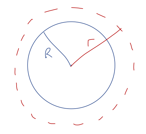
As we've already argued, symmetry tells us immediately that \( \vec{g}(\vec{r}) = g(r) \hat{r} \) in the case of a spherical source. Since \( d\vec{A} \) is also in the \( \hat{r} \) direction for a spherical surface, we have \( \vec{g} \cdot d\vec{A} = g(r) \), which we can pull out of the integral as we saw above. Thus,
\[ \begin{aligned} \oint_{\partial V} \vec{g} \cdot d\vec{A} = -4\pi G \int_V \rho(\vec{r}) dV \end{aligned} \]
becomes
\[ \begin{aligned} 4\pi g(r) r^2 = -4\pi G M \Rightarrow g(r) = -\frac{GM}{r^2}. \end{aligned} \]
This was way easier to find using Gauss's law than the direct calculation we did! What about inside the spherical shell? For \( r < R \), we again take a spherical surface:
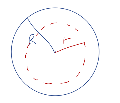
The entire calculation is the same as outside the sphere, except that now \( M_{\rm enc} \) is always zero - correspondingly, we simply have
\[ \begin{aligned} g(r) = 0 \end{aligned} \]
for \( r < R \). This again matches the result we found the hard way before - constant potential, which gives zero \( \vec{g} \) field when we take the gradient.
There aren't a huge number of applications of Gauss's law, in fact; the only three Gaussian surfaces that are commonly used are the sphere, the cylinder, and the box, matching problems with the corresponding symmetries (a sphere, a cylinder, or an infinite plane.) We will see one more very important application soon, when we talk about dark matter. In the rare cases where it does apply, it makes calculating \( \vec{g} \) really easy!
Comparison: gravity vs. electric force
You should recognize a lot of similarities between how we're dealing with the gravitational force and how you've seen the electric force treated before. Here's a quick list of equivalences between gravity and electric force:
Gravity vs. electric:
- Force: \( \vec{F}_g = -\frac{GMm}{r^2} \hat{r} \) vs. \( \vec{F}_e = +\frac{kQq}{r^2} \hat{r} \)
- Field: \( \vec{g} = \frac{\vec{F}_g}{m} = -\frac{GM}{r^2} \hat{r} \) vs. \( \vec{E} = \frac{F_e}{q} = \frac{kQ}{r^2} \hat{r} \)
- Potential energy: \( U(r) = -\frac{GMm}{r} \) vs. \( U(r) = +\frac{kQq}{r} \)
- Potential: \( \Phi = \frac{U}{m} = -\frac{GM}{r} \) vs. \( V = \frac{U}{q} = +\frac{kQ}{r} \)
and of course Gauss's law: for gravity we have
\[ \begin{aligned} \oint_{\partial V} \vec{g} \cdot d\vec{A}' = -4\pi G \int_V \rho(\vec{r}') dV' = -4\pi G M_{\rm enc}. \end{aligned} \]
while the electric version reads
\[ \begin{aligned} \oint_{\partial V} \vec{E} \cdot d\vec{A}' = +4\pi k Q_{\rm enc}. \end{aligned} \]
Notice how everything is almost completely identical! The main differences are a different constant (\( G \) vs. \( k \)), a different "charge" (\( m \) and \( M \) vs. \( q \) and \( Q \)), and the minus sign - reflecting the fact that like charges repel in electromagnetism, but they attract for gravity.
A lot of the tools and techniques we're talking about now will transfer more or less directly to electromagnetism; for example, calculating the electric potential \( V(\vec{r}) \) from an extended charged object.
Selected modern topics in gravity
One of the more exciting things about teaching gravitation is that we now have the tools to make contact with some really important and cutting-edge ideas in physics! I'll give you a taste of two such topics: effective theories, and dark matter.
Effective theory and gravity at the Earth's surface
As we've just seen, to the extent that the Earth is a sphere, we know that its gravitational field on the surface and above is
\[ \begin{aligned} \vec{g}(r) = -\frac{GM}{r^2} \hat{r}. \end{aligned} \]
However, this is not the form you use in the lab! For experiments on the Earth's surface, we replace this with the constant acceleration \( g \). In fact, we can derive this by expanding our more general result in the limit that we're pretty close to the Earth's surface.
Let \( R_E \) be the radius of the Earth, \( M_E \) its mass, and suppose that we conduct an experiment at a distance \( z \) above that radius. Then we have
\[ \begin{aligned} \vec{g}(z) = -\frac{GM_E}{(R_E+z)^2} \hat{z} = -g(z) \hat{z} \end{aligned} \]
where I've replaced \( \hat{r} \) with \( \hat{z} \), because if we're on the surface of a sphere, "up" is the same as the outwards radial direction. Now, if we assume that we're relatively close to the surface so \( z \ll R_E \), then a series expansion makes sense:
\[ \begin{aligned} g(z) = \frac{GM_E}{R_E^2 (1 + (z/R_E))^2 } = \frac{GM_E}{R_E^2} \left[ 1 - \frac{2z}{R_E} + \frac{3z^2}{R_E^2} + ... \right] \end{aligned} \]
We see that indeed, so long as \( z \) is very small compared to \( R_E \), then \( g(z) \approx g \), a constant acceleration. We can also see now where \( g \) comes from in terms of other constants; if we measure \( g \approx 9.8 {\rm m}/{\rm s}^2 \), and we also know \( G = 6.67 \times 10^{-11} {\rm m}^3 / {\rm kg} / {\rm s}^2 \) and \( R_E \approx 6400 \) km \( = 6.4 \times 10^6 \) m, then we can find the mass of the Earth:
\[ \begin{aligned} M_E = \frac{gR_E^2}{G} \approx 6 \times 10^{24}\ {\rm kg}. \end{aligned} \]
This is, essentially, the only way we have to measure \( M_E \); the composition of the Earth is complicated and not well-understood beyond the upper layers that we can look at directly, so it's hard to estimate using density times volume.
Our series expansion buys us a lot more than just estimating \( g \)! In particular, we have a specific prediction that if we change \( z \) by enough, we'll be sensitive to a correction term linear in \( z \)
\[ \begin{aligned} g(z) \approx g \left(1 - \frac{2z}{R_E} + ... \right) \end{aligned} \]
Boulder is about 1.6km above sea level, so in this formula, we would predict that \( g \) is smaller by about 0.05% due to our increased height. This is a very small difference, but not so small that it can't be measured! (Although there are other effects of similar size, including centrifugal force due to the fact that the Earth is spinning.)
Now we come to the big idea here, which is the idea of effective theory. This is something which is rarely taught in undergraduate physics, but I believe it's one of the most important ideas in physics - and it's lurking in a lot of what you are taught, even if we don't acknowledge it by name.
My definition of an effective theory is that it is a physical theory which intentionally ignores the true underlying physical model, on the basis of identifying a scale separation. If we are interested in some system of size \( r \), then any physics relevant at much longer scales \( L \gg r \) is "separated". So is any physics relevant at much shorter scales, \( \ell \ll r \).
Going back to our example for \( g(z) \), we could also ask about the influence of the Sun's gravity on an object on the Earth's surface; this would depend on the Earth-Sun distance, \( R_{ES} = 1.48 \times 10^{11} \) m. Or maybe we're worried about the quantum theory of gravity, and want to know the effect of corrections that occur at very short distances (our best modern estimate of the length scale at which this would matter is the Planck length, \( \ell_P = 1.6 \times 10^{-35} \) m.) Scale separation tells us that we can series expand such contributions in ratio to the scale \( z \) at which we're experimenting:
\[ \begin{aligned} g(z) \approx g \left( 1 - \frac{2z}{R_E} + ... \right) + C_1 \frac{z}{R_{ES}} + C_2 \frac{\ell_P}{z} + ... \end{aligned} \]
and although we can keep these terms in our expansion, as long as the numerical coefficients \( C_1, C2 \) aren't incredibly, surprisingly large, the ratios \( z/R{ES} \) and \( \ell_P/z \) are so incredibly small that we can always ignore such effects. So we can see the power of scale separation: large enough separation allows us to completely neglect other scales, because even their leading contribution in a series expansion would be tiny!
This validates the effective theory framework of ignoring any physical effects that are sufficiently well-separated, although it's very important to note that this depends on \( z \), the experimental scale. An effective theory doesn't claim to be the right and final answer: it's only "effective" for a certain well-defined set of experiments. If our \( z \) approaches any one of these other scales, then the series expansion relying on scale separation will break down, and we'll have to include the new physics at that scale to get the right answer.
A couple of slightly technical points I should make on the last equation I wrote. You might wonder why I can assume the series expansion for something like the Earth-Sun distance starts at \( z/R_{ES} \). Why can't there be an \( R_{ES} / z \) term, for example? That wouldn't make any physical sense, basically - it would imply that there's a large effect from the Earth-Sun distance in the limit that \( R_{ES} \) goes to infinity. We can't have a \( \ell_P/z \) term for a similar reason - it makes no sense as \( \ell_P \) goes away (goes to zero.)
Next time: we'll finish the discussion of effective theory, and on to dark matter!