For expanding around equilibrium, the SHO is all we need, and we've solved it thoroughly at this point. However, it turns out there's a lot of interesting physics and math in variations of the harmonic oscillator that have nothing to do with equilibrium expansion or energy conservation.
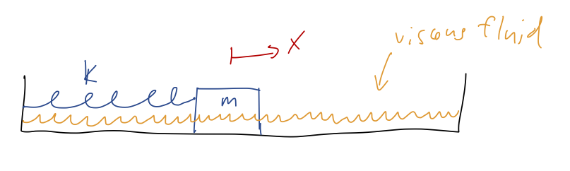
We'll begin our study with the damped harmonic oscillator. Damping refers to energy loss, so the physical context of this example is a spring with some additional non-conservative force acting. Specifically, what people usually call "the damped harmonic oscillator" has a force which is linear in the speed, giving rise to the equation
\[ \begin{aligned} m \ddot{x} = - b\dot{x} - kx. \end{aligned} \]
The new force is the familiar linear drag force, so we can imagine this to be the equation describing a mass on a spring which is sliding through a high-viscosity fluid, like molasses:
As Taylor observes, another very important instance of this equation is the LRC circuit, which contains an inductor, a resistor, and a capacitor in series. The differential equation for the charge in such a circuit is
\[ \begin{aligned} L\ddot{Q} + R\dot{Q} + \frac{Q}{C} = 0. \end{aligned} \]
Since this is not a circuits class I won't dwell on this example, but I point it out for those of you who might be more familiar with circuit equations.
Let's rearrange the equation of motion slightly and divide out by the mass, as we did for the SHO:
\[ \begin{aligned} \ddot{x} + 2\beta \dot{x} + \omega_0^2 x = 0 \end{aligned} \]
where
\[ \begin{aligned} \beta = \frac{b}{2m},\ \ \omega_0 = \sqrt{\frac{k}{m}}, \end{aligned} \]
using the conventional notation for this problem. The frequency \( \omega_0 \) is called the natural frequency; as we can see, it is the frequency at which the system would oscillate if we removed the damping term by setting \( b=0 \). The other constant \( \beta \) is called the damping constant, and it is proportional to the strength of the drag force. \( \beta \) has the same units as \( \omega_0 \), i.e. frequency or 1/time.
Once again, we have a linear, second-order, homogeneous ODE - so we just need to find two independent solutions to put together. Unfortunately, it's a little harder to guess what the solutions will be just by inspection this time. There is a more systematic way to find the answer, using the language of linear operators; the reading I assigned in Boas covers this method.
Instead, I'll follow what Taylor does and use the physicist's method of guess and check: we'll guess that a complex exponential solution will work here, just like in the regular SHO. Let's suppose that
\[ \begin{aligned} x(t) = e^{rt} \end{aligned} \]
and then plug in to find
\[ \begin{aligned} r^2 e^{rt} + 2\beta r e^{rt} + \omega_0^2 e^{rt} = 0. \end{aligned} \]
You can see right away why this was a good guess; every term has an \( e^{rt} \) that we can cancel off, and we're left with a quadratic equation for \( r \),
\[ \begin{aligned} r^2 + 2\beta r + \omega_0^2 = 0. \end{aligned} \]
We know how to solve this: the roots are
\[ \begin{aligned} r_{\pm} = -\beta \pm \sqrt{\beta^2 - \omega_0^2}. \end{aligned} \]
Two roots is perfect, since we need two independent functions for our general solution! So we immediately see that
\[ \begin{aligned} x(t) = C_1 e^{r_+ t} + C_2 e^{r_- t} \\ = C_1 e^{-\beta t + \sqrt{\beta^2 - \omega_0^2} t} + C_2 e^{-\beta t - \sqrt{\beta^2 - \omega_0^2} t} \\ = e^{-\beta t} \left( C_1 e^{\sqrt{\beta^2 - \omega_0^2} t} + C_2 e^{-\sqrt{\beta^2 - \omega_0^2}t} \right). \end{aligned} \]
(There is one subtlety here: if \( r_+ = r_- \), then we have actually only found one solution. I'll return to this case a little later.)
If we plug in \( \beta = 0 \) as a check, then we get \( \sqrt{-\omega_0^2} t = i\omega_0 t \) inside both of the exponentials in the second factor, giving back our undamped SHO solution as it should.
It should be obvious from looking at this that the relative size of \( \beta \) and \( \omega_0 \) will be very important in the qualitative behavior of these solutions: the exponentials inside the parentheses can be either real or imaginary as we change \( \beta \) relative to \( \omega_0 \). Let's go through the possibilities.
Damping strength and behavior of the damped SHO
Since we already know what happens at \( \beta = 0 \), let's start with small \( \beta \) and turn the strength of the force up from there. (\( \beta \) is dimensionless, so by "small \( \beta \)" I of course mean "small \( \beta/\omega_0 \).") In particular, as long as \( \beta < \omega_0 \), the combination \( \beta^2 - \omega_0^2 \) under the roots will always be negative. We define a new frequency \( \omega \) as follows:
\[ \begin{aligned} \sqrt{\beta^2 - \omega_0^2} = i \sqrt{\omega_0^2 - \beta^2} = i \omega. \end{aligned} \]
(Taylor calls this "\( \omega_1 \)", but the subscript 1 seems weird and confusing to me, so I'm deviating from his notation a little.) With this definition, we have for the overall solution
\[ \begin{aligned} x(t) = e^{-\beta t} \left(C_1 e^{i\omega t} + C_2 e^{-i\omega t} \right), \end{aligned} \]
or doing the same trick to combine the trig functions as before,
\[ \begin{aligned} x(t) = Ae^{-\beta t} \cos (\omega t - \delta). \end{aligned} \]
So we once again have an oscillating solution, almost the same as the SHO, except the amplitude dies off exponentially as \( e^{-\beta t} \). If we plot this, we can imagine an exponential "envelope" given by \( \pm Ae^{-\beta t} \), with the actual solution oscillating back and forth between the sides of the envelope:
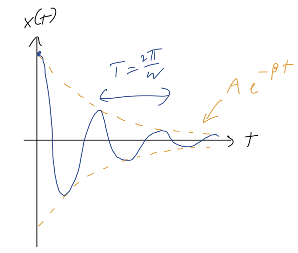
Note that this is no longer periodic, but the distance between maxima or minima within the envelope is still \( \tau = 2\pi / \omega \). If \( \beta \ll \omega_0 \), then we notice that \( \omega \approx \omega_0 \), so for very small damping the oscillation frequency is roughly the same as the natural oscillation.
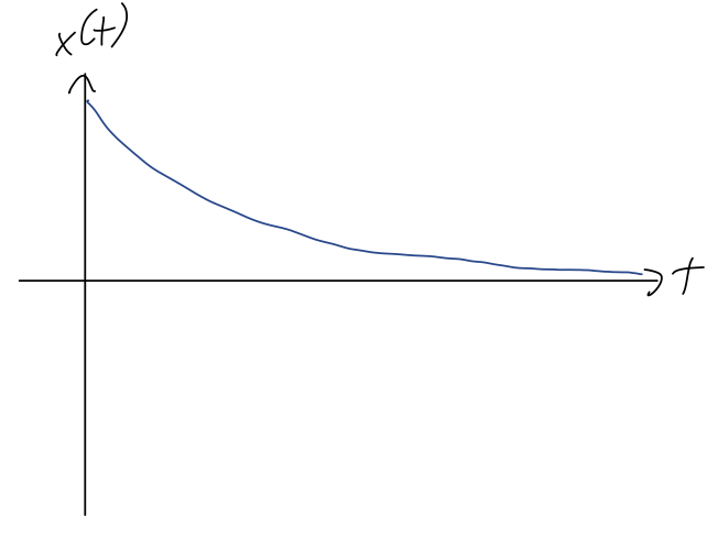
Let's move on to the case where \( \beta > \omega_0 \) - exact equality is tricky, so we'll do that last. In this case, all of the exponentials stay real, and we have
\[ \begin{aligned} x(t) = C_1 e^{-(\beta - \sqrt{\beta^2 - \omega_0^2}) t} + C_2 e^{-(\beta + \sqrt{\beta^2 - \omega_0^2}) t}. \end{aligned} \]
Since \( \sqrt{\beta^2 - \omega_0^2} < \beta \) given our assumptions, both terms decay exponentially in time, and there's no oscillation at all. Here's a sketch of this solution:
It's instructive to factor out the first exponential term completely from our solution:
\[ \begin{aligned} x(t) = e^{-(\beta - \sqrt{\beta^2 - \omega_0^2}) t} \left( C_1 + C_2 e^{-2\sqrt{\beta^2 - \omega_0^2} t}\right). \end{aligned} \]
As \( t \) increases, the second term here is negligible for the long-term behavior of the system, unless we have \( C_1 = 0 \). Let's match initial conditions to see what that would require:
\[ \begin{aligned} x_0 = x(0) = C_1 + C_2 \\ v_0 = \dot{x}(0) = -(\beta - \sqrt{\beta^2 - \omega_0^2}) C_1 - (\beta + \sqrt{\beta^2 - \omega_0^2}) C_2 \end{aligned} \]
We can solve this for \( C_1 = 0 \), and a bit of algebra reveals that it requires a specific relationship between \( v_0 \) and \( x_0 \),
\[ \begin{aligned} \frac{v_0}{x_0} = -(\beta + \sqrt{\beta^2 - \omega_0^2}). \end{aligned} \]
In particular, the minus sign tells us that this is only possible if \( v_0 \) and \( x_0 \) are in opposite directions. Aside from this rather special case, we can in general ignore the \( C_2 \) term completely at large \( t \), finding that
\[ \begin{aligned} x(t) \rightarrow C_1 e^{-\alpha t} \end{aligned} \]
defining the decay parameter \( \alpha \) as the coefficient in the exponential decay of the max amplitude at large \( t \), in this case
\[ \begin{aligned} \alpha = \beta - \sqrt{\beta^2 - \omega_0^2}. \end{aligned} \]
This solution exhibits some rather counterintuitive behavior: as we increase the strength of the damping force \( \beta \), the decay parameter \( \alpha \) actually becomes smaller, approaching \( \alpha = 0 \) as \( \beta \rightarrow \infty \)! To make sense of this, let's remember that the net force on our oscillator is
\[ \begin{aligned} F_{\rm net} = F_{\rm drag} + F_{\rm spring} = -2m\beta \dot{x} - k x \end{aligned} \]
Both forces push our object back towards the origin. But if \( \beta \) is extremely large, then there is an enormous force even if we try to move at a relatively small speed, so it will take much longer in time for us to actually get to the origin. We still get there eventually, because the \( -kx \) spring force always keeps pulling us to the origin as long as \( x \) is non-zero.
Let's come back to the third possibility, which is \( \beta = \omega_0 \). If we go back to our original solution, this gives us
\[ \begin{aligned} x(t) = C_1 e^{-(\beta - \sqrt{\beta^2 - \omega_0^2}) t} + C_2 e^{-(\beta + \sqrt{\beta^2 - \omega_0^2}) t} \rightarrow C_1 e^{-\beta t} + C_2 e^{-\beta t}. \end{aligned} \]
Now we only have one solution, repeated twice! This means our solution is suddenly incomplete: we need two independent functions to add together to have a general solution. To find a second solution, since this is clearly a special case, let's go back to the original differential equation and see what happens if \( \beta = \omega_0 \):
\[ \begin{aligned} \ddot{x} + 2 \beta \dot{x} + \beta^2 x = 0 \end{aligned} \]
Clearly \( e^{-\beta t} \) indeed works as a solution. To see the other one, we notice that we can rewrite the ODE as follows:
\[ \begin{aligned} \left( \frac{d^2}{dt^2} + 2\beta \frac{d}{dt} + \beta^2 \right) x(t) = 0 \end{aligned} \]
which can then be factorized,
\[ \begin{aligned} \left( D + \beta \right) \left( D + \beta \right) x(t) = 0. \end{aligned} \]
where I've replaced \( d/dt \) with the shorthand \( D \). (Expand it back out to convince yourself!) Doing algebra on \( d/dt \) like this works because of the distributive properties of \( d/dt \); the technical math term is that \( d/dt \) is a linear operator. Prof. Pollock has gone over some of this with you in his guest lectures. So, one way that this equation can be satisfied is just if
\[ \begin{aligned} \left( D + \beta \right) x(t) = 0, \end{aligned} \]
which matches on to our solution \( e^{-\beta t} \). But the other possibility is that this combination isn't zero: let's call it
\[ \begin{aligned} \left( D + \beta \right) x(t) = u(t) \neq 0. \end{aligned} \]
Then we're left with another first-order ODE,
\[ \begin{aligned} \left( D + \beta \right) u(t) = 0. \end{aligned} \]
So \( u(t) = C e^{-\beta t} \), but now we have to work backwards a bit:
\[ \begin{aligned} \left( D + \beta \right) x(t) = C e^{-\beta t} \end{aligned} \]
We can use the general first-order solution in Boas to find the answer directly, but if you stare at this for a minute, you might think to try the following combination: if
\[ \begin{aligned} x(t) = C t e^{-\beta t} \end{aligned} \]
then
\[ \begin{aligned} \frac{dx}{dt} = C e^{-\beta t} - \beta C t e^{-\beta t} \end{aligned} \]
so the \( te^{-\beta t} \) will cancel out, matching the right-hand side. Thus, the general solution in this special case where \( \beta = \omega_0 \) is
\[ \begin{aligned} x(t) = C_1 e^{-\beta t} + C_2 t e^{-\beta t}. \end{aligned} \]
Once again, we see no oscillations - everything is pure exponential decay, but with an extra factor of \( t \) that only matters at small times. Once again as \( t \) becomes very large, the amplitude decays exponentially proportional to \( \beta \).
Let's summarize all of our solutions:
- If \( \beta < \omega_0 \), the system is said to be underdamped. Our solution takes the form
\[ \begin{aligned} x(t) = Ae^{-\beta t} \cos (\omega t - \delta), \end{aligned} \]
with oscillations, and the overall amplitude decaying with decay parameter \( \alpha = \beta \).
- If \( \beta = \omega_0 \), the system is critically damped. We have the funny solution we just found,
\[ \begin{aligned} x(t) = C_1 e^{-\beta t} + C_2 t e^{-\beta t}, \end{aligned} \]
with no oscillations and again the ampltiude at large times decaying exponentially with \( \alpha = \beta \).
- Finally, if \( \beta > \omega_0 \), the system is overdamped. In this case the general solution looks like
\[ \begin{aligned} x(t) = C_1 e^{-(\beta - \sqrt{\beta^2 - \omega_0^2}) t} + C_2 e^{-(\beta + \sqrt{\beta^2 - \omega_0^2}) t}. \end{aligned} \]
again pure exponential decay, but this time with decay parameter \( \alpha = \beta - \sqrt{\beta^2 - \omega_0^2} \), which goes to zero as \( \beta \) gets larger and larger.
We can sketch the size of the decay parameter vs. the damping parameter \( \beta \):

When designing a system that behaves like a damped oscillator, this tells us that it's actually optimal to tune \( \beta \) (or \( \omega_0 \)) so that the system is as close to critical as possible. A good example is shock absorbers in a car, which are designed to damp out the oscillations transferred from the road to the passengers.