There's one more really important generalization we can add to the damped harmonic oscillator, which is a driving force. The damped oscillator is sort of a special case, because with no energy input the damping will quickly dispose of all the mechanical energy and cause the oscillator to stop. In many realistic applications (like a clock), we want an oscillator that will continue to oscillate, which means an external force has to be applied.
We'll assume the applied force depends on time, but not on the position of the oscillator, so it takes the general form \( F(t) \). Then the ODE becomes
\[ \begin{aligned} m \ddot{x} + b \dot{x} + kx = F(t). \end{aligned} \]
(Again, if you're familiar with circuits, this is like an LRC circuit adding in a source of electromotive force like a battery.)
With the addition of the driving force, our ODE is no longer homogeneous. This means that we no longer have the principle of superposition: we can't find our general solution by just taking any two independent solutions and adding them together with constants.
Instead, we can use an old technique that we've seen for first-order equations. Suppose that we find a function \( x_c(t) \), the complementary solution, that just gives zero when plugged in to the left-hand side of the ODE, i.e.
\[ \begin{aligned} m \ddot{x}_c + b \dot{x}_c + kx_c = 0. \end{aligned} \]
(This equation with the non-homogeneous part thrown out is called the complementary equation.) Next, we find a function \( x_p(t) \) called the particular solution, which satisfies the full equation:
\[ \begin{aligned} m\ddot{x}_p + b\dot{x}_p + kx_p = F(t). \end{aligned} \]
Although the particular solution works, since this is a linear second-order ODE, we know that the general solution requires two undetermined constants. We can't add any constants to \( x_p \) itself; for example, \( 2x_p(t) \) is not a solution since it gives \( 2F(t) \) on the right-hand side. But since the complementary solution gives zero, we can add that in with an unknown constant.
Thus, the full general solution is
\[ \begin{aligned} x(t) = C_1 x_{1,c}(t) + C_2 x_{2,c}(t) + x_p(t) \end{aligned} \]
The good news is that we've already found the complementary solutions, since the complementary equation is just the regular damped oscillator that we just finished solving.
How we find the particular solution depends strongly on what the non-homogeneous part of the equation looks like. Constant is the simplest possibility: let's do a quick example to demonstrate.
Exercise: non-homogeneous with constant driving
Find the general solution of the equation:
\[ \begin{aligned} \ddot{y} - \dot{y} - 6y = 4 \end{aligned} \]
(As always, give this a try yourself before you read my answer!) We start with the complementary equation,
\[ \begin{aligned} \ddot{y}_c - \dot{y}_c - 6y_c = 0 \end{aligned} \]
We can solve this using the algebra of differential operators: rewriting the complementary equation gives
\[ \begin{aligned} (D^2 - D - 6) y_c = 0 \end{aligned} \]
which we can factorize into
\[ \begin{aligned} (D+2)(D-3)y_c = 0. \end{aligned} \]
As usual we can write a simple exponential solution for each monomial:
\[ \begin{aligned} y_{1,c}(t) = e^{-2t},\ \ y_{2,c}(t) = e^{+3t}. \end{aligned} \]
On to the particular solution. We always want to look for a particular solution that has a similar form to the driving. A constant particular solution is especially nice, since all of the derivatives vanish immediately. It should be easy to see right away that
\[ \begin{aligned} y_p(t) = -\frac{2}{3} \end{aligned} \]
will satisfy the equation. Thus, putting everything together, we have for the general solution
\[ \begin{aligned} y(t) = C_1 e^{-2t} + C_2 e^{+3t} - \frac{2}{3}. \end{aligned} \]
Coming back to the specific case of the oscillator, suppose that wehave a constant driving force \( F(t) = F_0 \). Rewriting the equation into our standard form,
\[ \begin{aligned} \ddot{x} + 2\beta \dot{x} + \omega_0^2 x = \frac{F_0}{m} \end{aligned} \]
so to our damped oscillator solutions from before, we simply have to add the particular solution
\[ \begin{aligned} x_p(t) = \frac{F_0}{m \omega_0^2}. \end{aligned} \]
This is just a constant offset to our \( x \) coordinate. So, for example, if we take an oscillator moving horizontally and reorient it so that it's hanging vertically subject to gravity, the motion will be exactly the same except that the equilibrium position will be displaced to
\[ \begin{aligned} x_p = \frac{g}{\omega_0^2} = \frac{mg}{k} \end{aligned} \]
(which is exactly the new equilibrium point where the spring force \( kx_p \) balances the gravitational force \( mg \).)
Let's do a more interesting example of a driving force.
Complex exponential driving
Now we'll assume a driving force of exponential form:
\[ \begin{aligned} F(t) = F_0 e^{ct} \end{aligned} \]
where \( c \) can be complex. This covers both regular exponential forces (if \( c \) is real), as well as the very important case of oscillating driving force (if \( c \) is imaginary.)
The obvious thing to try for our particular solution is exactly the same form: we'll guess that
\[ \begin{aligned} x_p(t) = C_3 e^{ct} \end{aligned} \]
will give us a solution, and then try it out. Note that although I put in an unknown constant \( C_3 \), as we've seen with other particular solutions this is not an arbitrary constant; we expect only a specific choice of \( C_3 \) to work given a certain driving force.
Let's plug our guessed solution back in and see what we get: from
\[ \begin{aligned} \ddot{x} + 2\beta \dot{x} + \omega_0^2 x = \frac{F_0}{m} e^{ct} \end{aligned} \]
we have
\[ \begin{aligned} \left[ c^2 + 2\beta c + \omega_0^2 \right] C_3 e^{ct} = \frac{F_0}{m} e^{ct} \end{aligned} \]
or cancelling off the exponentials,
\[ \begin{aligned} C_3 = \frac{F_0}{m(c^2 + 2\beta c + \omega_0^2)}. \end{aligned} \]
Once again, this is not arbitrary! Both \( c \) and \( F_0 \) are given to us as part of the external driving force: they are literally numbers that are dialed in on whatever machine is providing the driving for our experiment.
Let's step back for a moment and look at the big picture. Remember that the complementary solutions take the form \( e^{r_{\pm} t} \), where \( r_{\pm} \) solve the equation
\[ \begin{aligned} r^2 + 2\beta r + \omega_0^2 = 0. \end{aligned} \]
The full solution is two complementary solutions with arbitrary coefficients, plus one particular:
\[ \begin{aligned} x(t) = C_+ e^{r_+ t} + C_- e^{r_- t} + C_3 e^{ct} \end{aligned} \]
with \( C_3 \) determined by \( F_0 \) and \( c \) as we found above. All of these exponents can be complex, so we can have individual contributions that oscillate at one, two, or three different frequencies; we'll make more sense of this soon.
Notice that there's an important edge case here: the same quadratic equation for \( r \) appears again in the denominator of \( C3 \). So if we have \( c = r{\pm} \), then our formula for \( C_3 \) blows up. This is similar to what happened in the critical damping case: our would-be particular solution fails, because it's not independent from the complementary solution. The way to fix this, similarly, is to take a particular solution of the form \( C_3 te^{ct} \) or \( C_3 t^2 e^{ct} \) as needed.
So far this is totally general, but let's specialize now to the very important case of an oscillating driving force, \( c = i \omega \). Plugging back in and splitting into real and imaginary parts in the denominator gives
\[ \begin{aligned} C_3 = \frac{F_0/m}{(\omega_0^2 - \omega^2) + 2i \beta \omega}. \end{aligned} \]
It will be useful to rewrite this in polar form, \( C_3 = Ae^{-i\delta} \). To find \( A \) first, we multiply by the complex conjugate:
\[ \begin{aligned} |C_3|^2 = \frac{F_0/m}{(\omega_0^2 - \omega^2) - 2i \beta \omega} \frac{F_0/m}{(\omega_0^2 - \omega^2) + 2i \beta \omega} \\ = \frac{F_0^2/m^2}{(\omega_0^2 - \omega^2)^2 + 4\beta^2 \omega^2}, \end{aligned} \]
so the amplitude is
\[ \begin{aligned} A = |C_3| = \frac{F_0/m}{\sqrt{(\omega_0^2 - \omega^2)^2 + 4\beta^2 \omega^2}}. \end{aligned} \]
To get the phase, we separate out the real and imaginary parts of our original expression, which means moving the factors of \( i \) upstairs:
\[ \begin{aligned} C_3 = \frac{F_0/m}{(\omega_0^2 - \omega^2) + 2i \beta \omega} \left[\frac{(\omega_0^2 - \omega^2) - 2i \beta \omega}{(\omega_0^2 - \omega^2) - 2i \beta \omega}\right] \\ = \frac{F_0/m}{(\omega_0^2 - \omega^2)^2 + 4\beta^2 \omega^2} \left[ (\omega_0^2 - \omega^2) - 2i \beta \omega \right]. \end{aligned} \]
The factor in front doesn't matter; the angle just depends on the relative size of the real and imaginary parts. We can make a quick sketch:
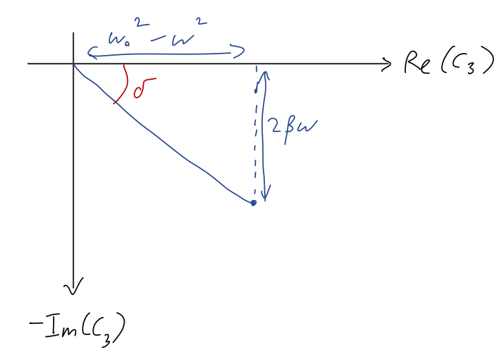
so that the complex phase is given by
\[ \begin{aligned} \tan \delta = \frac{2\beta \omega}{\omega_0^2 - \omega^2}. \end{aligned} \]
taking out a minus sign since we wrote this as \( Ae^{-i\delta} \) to begin with. Putting everything back together, our particular solution becomes
\[ \begin{aligned} x_p(t) = A e^{-i\delta} e^{i\omega t}. \end{aligned} \]
This has to be real since it's a position, so our solution is actually the real part,
\[ \begin{aligned} x_p(t) = \frac{F_0/m}{\sqrt{(\omega_0^2 - \omega^2)^2 + 4\beta^2 \omega^2}} \cos (\omega t - \delta). \end{aligned} \]
So the particular contribution oscillates at the driving frequency \( \omega \), and its amplitude depends most strongly on the relative size of the driving frequency \( \omega \) to the natural frequency \( \omega_0 \).