Finishing our discussion of resonances from last time: in addition to the height of the resonance peak, the width of the resonance is also an important quantity to know. We argued from our series expansion before that small \( \beta \) means narrower width, since the quadratic term in \( (\omega - \omega_0) \) gets steeper at smaller \( \beta \). Let's be a little more quantitative and ask about the full-width at half maximum, or FWHM. By convention, this is defined for the value of the squared amplitude, \( |A|^2 \) (which is proportional to the energy, recall: \( E = \frac{1}{2} k|A|^2 \).)
Let's be clever about this. Recall that the squared amplitude is equal to
\[ \begin{aligned} |A|^2 = \frac{F_0^2/m^2}{(\omega_0^2 - \omega^2)^2 + 4\beta^2 \omega^2}. \end{aligned} \]
Now, the peak occurs roughly where the first term vanishes, leaving just the second term. Therefore, the half-max value is where the first term is equal to the second term, so the denominator becomes \( 8\beta^2 \omega^2 \). Setting these equal gives
\[ \begin{aligned} (\omega_0^2 - \omega_{\rm HM}^2)^2 = 4\beta^2 \omega_{\rm HM}^2 \\ \omega_0^2 - \omega_{\rm HM}^2 \approx \pm 2\beta \omega_{\rm HM}. \end{aligned} \]
This is easy to solve since it's a quadratic equation, although we need to be a little careful with which roots we keep. Using the quadratic formula, we find
\[ \begin{aligned} \omega_{\rm HM} = \mp \beta \pm \sqrt{\beta^2 + \omega_0^2} \end{aligned} \]
(all four combinations of signs appear, because we have two minus signs and then two roots for each.) Now, since we're working where \( \beta \ll \omega_0 \), the \( \beta^2 \) under the root is completely negligible, and the second term is just \( \pm \omega_0 \). This must be \( +\omega0 \), in fact, because \( \omega{\rm HM} \) has to be positive. Thus, we find our approximate answer
\[ \begin{aligned} \omega_{\rm HM} = \omega_0 \pm \beta. \end{aligned} \]
So we see explicitly that at roughly a difference in frequency of \( \beta \) on either side of the peak, the squared amplitude is reduced by half. The smaller \( \beta \) is, the sharper our resonance peak will be (and the larger the peak amplitude will be, as we already found.)
Quality factor
One more quantity that is conventionally defined in the context of resonance is the quality factor or Q-factor, denoted by \( Q \). This is defined to be
\[ \begin{aligned} Q \equiv \frac{\omega_0}{2\beta} \end{aligned} \]
so it is a dimensionless number. This must be a number much larger than 1 under our assumptions, and the larger \( Q \) is, the sharper the resonance peak will be.
We can rewrite the peak resonance amplitude in terms of \( Q \): recall that we had
\[ \begin{aligned} |A| \approx \frac{F_0}{2m\omega_0 \beta} = \frac{F_0}{m\omega_0^2} Q. \end{aligned} \]
Essentially, \( Q \) is a comparison of the natural frequency of the resonator to the damping factor (which is, of course, also a frequency.) These correspond to two important physical timescales: \( T = 2\pi / \omega_0 \) determines the frequency of oscillation of the undriven oscillator, whereas since the amplitude dies off as \( e^{-\beta t} \) due to damping, \( \tau = 1/\beta \) gives the natural time for the decay of the amplitude. We can rewrite \( Q \) in terms of these timescales as
\[ \begin{aligned} Q = \frac{2\pi/T}{2/\tau} = \frac{\pi \tau}{T}. \end{aligned} \]
So a large \( Q \) means that a large number of oscillation periods \( T \) fit within a single decay time \( \tau \). In other words, if we turn the driving force off, a high-\( Q \) resonator will continue to oscillate for a long time, losing energy very slowly to the damping.
Let's summarize what we've found. (There is one more small observation we can make about the phase shift \( \delta \); it changes rapidly near a resonance. But I don't have much to say about the phase shift in this context, so I'll let you read about it in Taylor.) For a weakly damped driven oscillator, a resonance peak occurs for \( \omega_0 \approx \omega \). The amplitude at this peak is
\[ \begin{aligned} |A| \approx \frac{F_0}{2m\omega_0 \beta} = \frac{F_0}{m \omega_0^2} Q. \end{aligned} \]
The full-width at half-maximum is at approximately \( \omega = \omega_0 \pm \beta \). The peak location as a function of \( \omega \) is actually slightly to the left of \( \omega_0 \), at
\[ \begin{aligned} \omega = \omega_{\rm peak} = \sqrt{\omega_0^2 - 2\beta^2}. \end{aligned} \]
If instead we vary \( \omega_0 \) and hold \( \omega \) fixed, the resonance peak is exactly at \( \omega_0 = \omega \). Finally, this is all focused on the long-time behavior, i.e. just the particular solution! There is also a transient oscillation which occurs at short times; since we are in the underdamped regime, the frequency of the transient oscillations is
\[ \begin{aligned} \omega_1 = \sqrt{\omega_0^2 - \beta^2} \end{aligned} \]
(not to be confused with \( \omega_{\rm peak} \)!)
Fourier series
So far, we've only solved two particular cases of driving force for the harmonic oscillator: constant, and sinusoidal (i.e. complex exponential.) The latter case is useful on its own, since there are certainly cases in which this is a good model for a real driving force. But it's actually much more useful than it appears at first. This is thanks to a very powerful technique known as Fourier's method, or more commonly, Fourier series.
Let's think back to our earlier discussion of another important series method, which was power series. Recall that our starting point was to imagine a power-series representation of an arbitrary function \( f(x) \):
\[ \begin{aligned} f(x) = c_0 + c_1 x + c_2 x^2 + ... = \sum_{n=0}^{\infty} c_n x^n \end{aligned} \]
There are subtle mathematical issues about convergence and domain/range, as we noted. But putting the rigorous issues aside, the basic idea is that both sides of this equation are the same thing, hence the term "representation". If we really keep an infinite number of terms, there is no loss of information when we go to the series - it is the function \( f(x) \).
Our starting point for Fourier series is very similar. We suppose that we can write a Fourier series representation of an arbitrary function \( f(t) \):
\[ \begin{aligned} f(t) = \sum_{n=0}^\infty \left[ a_n \cos(n \omega t) + b_n \sin (n \omega t) \right], \end{aligned} \]
where we now have two sets of arbitrary coefficients \( a_n \) and \( b_n \), and \( \omega \) is a fixed angular frequency. Now, unlike the power-series representation, this actually can't work for any \( f(t) \); the issue is that since we're using sine and cosine, the series representation is now explicitly periodic, with period \( \tau = 2\pi / \omega \). So for both sides of this equation to be the same, we must require that the function \( f(t) \) is also periodic, i.e. this is valid only if
\[ \begin{aligned} f(t + \tau) = f(t). \end{aligned} \]
(In other words, \( \omega \) is not something we pick arbitrarily - it comes from the periodicity of the function \( f(t) \) we're trying to represent.) With this one important condition of periodicity, we now think of this just like a power-series representation: if we really keep an infinite number of terms, both sides of the equation are identical.
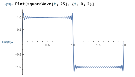
Two small, technical notes at this point. First, again if we went into detail on the mathematical side, we would find that there are certain requirements on the function \( f(t) \) for the Fourier series representation to converge properly - the function has to be "nice enough" for the series to work, roughly. The requirements for "nice enough" are weaker than you might expect; in particular, even sharp and discontinuous functions like a sawtooth or square wave admit Fourier series representations which converge at more or less every point. Here's the Fourier series for a square wave, truncated at the first 25 terms (which might sound like a lot, but is really easy for a computer to handle:)
Second, you might wonder why we use this particular form of the series. Why not a power series in only cosine with phase shifts, or a power series in \( \cos(\omega t)^n \) instead of \( \cos(n \omega t) \)? The short answer is that these wouldn't be any different - through trig identities, they're related to the form I've written above. The standard form that we'll be using makes it especially easy to calculate the coefficients \( a_n \) and \( b_n \) for a given function, as we shall see.
Now, in practice we can't really compute the entire infinite Fourier series except in really special cases. This is just like power series: after this formal setup, in practice we will use the truncated Fourier series
\[ \begin{aligned} f_M(t) = \sum_{n=0}^{M} \left[ a_n \cos(n \omega t) + b_n \sin (n \omega t) \right] \end{aligned} \]
and adjust \( M \) until the error made by truncation is small enough that we don't care about it.
Unlike power series, we don't need to come up with any fancy additional construction to find a useful Fourier series. In fact, the basic definition is enough to let us calculate the coefficients of the series for any function. To get there, we need to start by playing with some integrals!
Let's warm up with the following integral:
\[ \begin{aligned} \int_{-\tau/2}^{\tau/2} \cos (\omega t) dt = \left. \frac{1}{\omega} \sin (\omega t) \right|_{-\tau/2}^{\tau/2} \\ = \frac{1}{\omega} \left[ \sin\left( \frac{\omega \tau}{2} \right) - \sin\left( \frac{-\omega \tau}{2} \right) \right]. \end{aligned} \]
The fact that we've integrated over a single period lets us immediately simplify the result. By definition of the period, we know that
\[ \begin{aligned} \sin(\omega (t + \tau)) = \sin(\omega t + 2\pi) = \sin(\omega t). \end{aligned} \]
Since the difference between the two sine functions is exactly \( \omega \tau \), they are equal to each other and cancel perfectly. So the result of the integral is 0. Similarly, we would find that
\[ \begin{aligned} \int_{-\tau/2}^{\tau/2} \sin (\omega t) = 0. \end{aligned} \]
Both of these simple integrals are just stating the fact that over the course of a single period, both sine and cosine have exactly as much area above the axis as they do below the axis.
This is a simple observation, but it's important that we integrate for an entire period of oscillation to get zero as the result. (Some books will use the interval from \( 0 \) to \( \tau \) to define Fourier series instead, for example; everything we're about to do works just as well for that convention.)
Now, what if we start combining trig functions together? The graphical context above suggests that if we square the trig functions and then integrate, we will no longer get zero, because they'll be positive everywhere. Indeed, it's straightforward to show that
\[ \begin{aligned} \int_{-\tau/2}^{\tau/2} \sin (\omega t) \sin (\omega t) dt = \int_{-\tau/2}^{\tau/2} \cos (\omega t) \cos (\omega t) dt = \frac{\pi}{\omega} = \frac{\tau}{2} \end{aligned} \]
(I am writing \( \sin^2 \) and \( \cos^2 \) suggestively as a product of two sines and cosines.) However, if we have one sine and one cosine, we instead get
\[ \begin{aligned} \int_{-\tau/2}^{\tau/2} \sin (\omega t) \cos (\omega t) dt = \int_{-\tau/2}^{\tau/2} \frac{1}{2} \sin (2\omega t) dt = 0 \end{aligned} \]
(this is now integrating over two periods for \( \sin(2\omega t) \) - zero twice is still just zero!)
So far, so good. But what if we start combining trigonometric functions of the more general form \( \sin (n \omega t) \), as appears in our Fourier series expansion? For example, what is the result of the integral
\[ \begin{aligned} \int_{-\tau/2}^{\tau/2} \sin(3 \omega t) \sin(5 \omega t) dt = ? \end{aligned} \]
We could painstakingly apply trig identities to break this down into a number of integrals over \( \sin(\omega t) \) and \( \cos (\omega t) \). However, a much better way to approach this problem is using complex exponentials - which we'll do next time!