Our next important topic is something we've already run into a few times: oscillatory motion, which also goes by the name simple harmonic motion. This sort of motion is given by the solution of the simple harmonic oscillator (SHO) equation,
\[ \begin{aligned} m\ddot{x} = -kx \end{aligned} \]
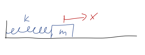
This happens to be the equation of motion for a spring, assuming we've put our equilibrium point at \( x=0 \):
The simple harmonic oscillator is an extremely important physical system study, because it appears almost everywhere in physics. In fact, we've already seen why it shows up everywhere: expansion around equilibrium points. If \( y_0 \) is an equilibrium point of \( U(y) \), then series expanding around that point gives
\[ \begin{aligned} U(y) = U(y_0) + \frac{1}{2} U''(y_0) (y-y_0)^2 + ... \end{aligned} \]
using the fact that \( U'(y_0) = 0 \), true for any equilibrium. If we change variables to \( x = y-y_0 \), and define \( k = U''(y_0) \), then this gives
\[ \begin{aligned} U(x) = U(x_0) + \frac{1}{2} kx^2 \end{aligned} \]
and then
\[ \begin{aligned} F(x) = -\frac{dU}{dx} = -kx \end{aligned} \]
which results in the simple harmonic oscillator equation. Since we're free to add an arbitrary constant to the potential energy, we'll ignore \( U(x_0) \) from now on, so the harmonic oscillator potential will just be \( U(x) = (1/2) kx^2 \).
Before we turn to solving the differential equation, let's remind ourselves of what we expect for the general motion using conservation of energy. Suppose we have a fixed total energy \( E \) somewhere above the minimum at \( E=0 \). Overlaying it onto the potential energy, we have:
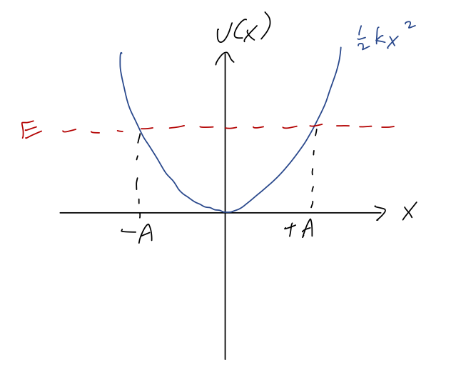
Because of the symmetry of the potential, if the value of \( x \) where \( E = U \) at positive \( x \) is \( U(A) = E \), then we must also have \( U(-A) = E \). Since these are the turning points, we see that \( A \), the amplitude, is the maximum possible distance that our object can reach from the equilibrium point; it must oscillate back and forth between \( x = \pm A \). We also know that \( T=0 \) at the turning points, which means that
\[ \begin{aligned} E = \frac{1}{2} kA^2. \end{aligned} \]
This relation will make it useful to write our solutions in terms of the amplitude. But to do that, first we have to find the solutions! It's conventional to rewrite the SHO equation in the form
\[ \begin{aligned} \ddot{x} = -\omega^2 x, \end{aligned} \]
where
\[ \begin{aligned} \omega^2 \equiv \frac{k}{m}. \end{aligned} \]
The combination \( \omega \) has units of 1/time, and the notation suggests it is an angular frequency - we'll see why shortly.
Solutions to the SHO equation
I've previously argued that just by inspection, we know that \( \sin(\omega t) \) and \( \cos(\omega t) \) solve this equation, because we need an \( x(t) \) that goes back to minus itself after two derivatives (and kicks out a factor of \( \omega^2 \).) But let's be more systematic this time.
Thinking back to our general theory of ODEs, we see that this equation is:
- Linear (no functions acting on \( x \))
- Second-order (double derivative on the left-hand side)
- Homogeneous (every time has an \( x \) or derivatives)
Since it's linear, we know there exists a general solution, and since it's second-order, we know it must contain exactly two unknown constants. We haven't talked about the importance of homogeneous and second-order yet, so let's look at that now. The most general possible homogeneous, linear, second-order ODE takes the form
\[ \begin{aligned} \frac{d^2y}{dx^2} + P(x) \frac{dy}{dx} + Q(x) y(x) = 0, \end{aligned} \]
where \( P(x) \) and \( Q(x) \) are arbitrary functions of \( x \). All solutions of this equation for \( y(x) \) have an extremely useful property known as the superposition principle: if \( y_1(x) \) and \( y_2(x) \) are solutions, then any linear combination of the form \( ay_1(x) + by_2(x) \) is also a solution. It's easy to show that if you plug that combination in to the ODE above, a bit of algebra gives
\[ \begin{aligned} a \left( \frac{d^2y_1}{dx^2} + P(x) \frac{dy_1}{dx} + Q(x) y_1(x) \right) + b \left( \frac{d^2y_2}{dx^2} + P(x) \frac{dy_2}{dx} + Q(x) y_2(x) \right) = 0 \end{aligned} \]
and since by assumption both \( y_1 \) and \( y_2 \) are solutions of the original equations, both of the expressions in parentheses are 0, so the whole left-hand side is 0 and the equation is true. Notice that the homogeneous part is very important for this: if there was some other \( F(x) \) on the right-hand side of the original equation, then we would get \( aF(x) + bF(x) \) on the left-hand side for our linear combination, and superposition will not work.
Anyway, the superposition principle greatly simplifies our search for a solution: if we find any two solutions, then we can add them together with arbitrary constants and we have the general solution. Let's go back to the SHO equation:
\[ \begin{aligned} \ddot{x} = - \omega^2 x \end{aligned} \]
As I mentioned before, two functions that both satisfy this equation are \( \sin(\omega t) \) and \( \cos(\omega t) \). So the general solution, by superposition, is
\[ \begin{aligned} x(t) = B_1 \cos (\omega t) + B_2 \sin (\omega t). \end{aligned} \]
This is indeed oscillatory motion, since both \( \sin \) and \( \cos \) are periodic functions: specifically, if we wait for \( t = \tau = 2\pi / \omega \), then
\[ \begin{aligned} x(t+\tau) = B_1 \cos (\omega t + 2\pi) + B_2 \sin (\omega t + 2\pi) = B_1 \cos (\omega t) + B_2 \sin (\omega t) = x(t) \end{aligned} \]
i.e. after a time of \( \tau \), the system returns to exactly where it was. The time length \( \tau \) is known as the period of oscillation, and we see that indeed \( \omega \) is the corresponding angular frequency.
To fix the arbitrary constants, we would just need to plug in initial conditions. If we have an initial position \( x_0 \) and initial speed \( v_0 \), then plugging in at \( t=0 \) the sine always vanishes, and we get the simple system of equations
\[ \begin{aligned} x_0 = x(0) = B_1 \\ v_0 = \dot{x}(0) = B_2 \omega \end{aligned} \]
so
\[ \begin{aligned} x(t) = x_0 \cos (\omega t) + \frac{v_0}{\omega} \sin (\omega t). \end{aligned} \]
This is a perfectly good solution, but this way of writing it makes answering certain questions inconvenient. For example, what is the amplitude \( A \), i.e. the maximum displacement from \( x=0 \)? It's possible to solve for, but certainly not obvious.
Instead of trying to find \( A \) directly, we'll just rewrite our general solution in a different form. We know that trig identities let us combine sums of sine and cosine into a single trig function. Thus, the general solution must also be writable in the form
\[ \begin{aligned} x(t) = A \cos (\omega t - \delta) \end{aligned} \]
where now \( A \) and \( \delta \) are the arbitrary constants. In this form, it's easy to see that \( A \) is exactly the amplitude, since the maximum of a single trig function is at \( \pm 1 \). We could relate \( A \) and \( \delta \) back to \( B_1 \) and \( B_2 \) using trig identities (look in Taylor), but instead we can just re-apply the initial conditions to this form:
\[ \begin{aligned} x_0 = x(0) = A \cos (-\delta) = A \cos \delta \\ v_0 = \dot{x}(0) = -\omega A \sin(-\delta) = \omega A \sin \delta \end{aligned} \]
using trig identities to simplify. (We used \( -\delta \) instead of \( +\delta \) inside our general solution to ensure that there are no minus signs in these equations, in fact.) To compare a little more closely between forms, we see that if we start from rest and at positive \( x_0 \), we must have \( \delta = 0 \) and so
\[ \begin{aligned} x(t) = A \cos (\omega t) = x_0 \cos (\omega t). \end{aligned} \]
On the other hand, if we start at \( x=0 \) but with a positive initial speed \( v_0 \), we must have \( \delta = \pi/2 \) to match on, and so
\[ \begin{aligned} x(t) = A \cos \left(\omega t - \frac{\pi}{2}\right) = A \sin (\omega t) = \frac{v_0}{\omega} \sin (\omega t). \end{aligned} \]
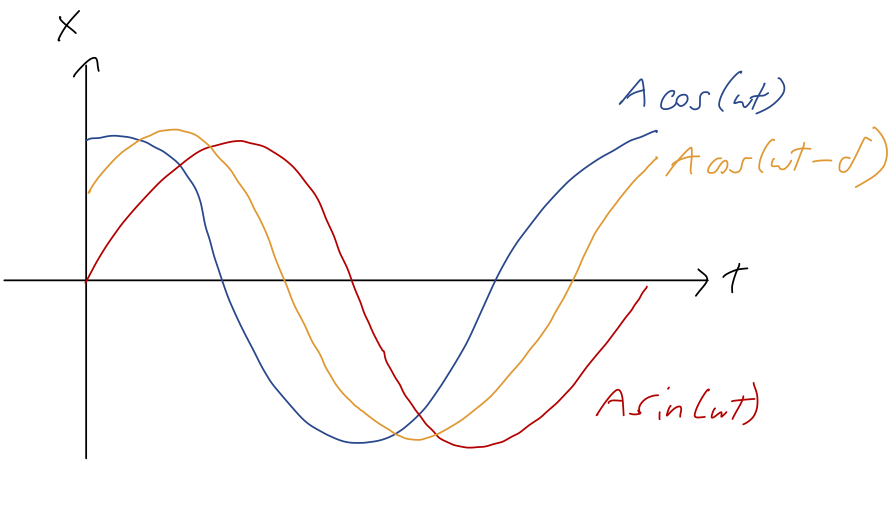
In between the pure-cosine and pure-sine cases, for \( \delta \) between 0 and \( \pi/2 \), we have that both position and speed are non-zero at \( t=0 \). We can visualize the resulting motion as simply a phase-shifted version of the simple cases, with the phase shift \( \delta \) determining the offset between the initial time and the time where \( x=A \):
Earlier, we found that the amplitude is related to the total energy as \( E = \frac{1}{2} kA^2 \). We can verify this against our solutions with an \( A \) in them: if we start at \( x=A \) from rest, then
\[ \begin{aligned} E = U_0 = \frac{1}{2} kx(0)^2 = \frac{1}{2} k A^2 \end{aligned} \]
and if we start at \( x=0 \) (so \( U=0 \)) at speed \( v_0 \), then
\[ \begin{aligned} E = T_0 = \frac{1}{2} mv_0^2 = \frac{1}{2} kA^2 \\ A = \sqrt{\frac{m}{k}} v_0 = \frac{v_0}{\omega} \end{aligned} \]
which matches what we found above comparing our two solution forms. In fact, it's easy to show using the phase-shifted cosine solution that \( E = \frac{1}{2}kA^2 \) always - I won't go through the derivation, but it's in Taylor.
We're not quite done yet: there is actually yet another way to write the general solution, which will just look like a rearrangement for now but will be extremely useful when we add extra forces to the problem. But to understand it, we need to take a brief math detour into the complex numbers.
Complex numbers
This is one of those topics that I suspect many of you have seen before, but you might be rusty on the details. So I will go quickly over the basics; if you haven't seen this recently, make sure to go carefully through the assigned reading in Boas.
Complex numbers are an important and useful extension of the real numbers. In particular, they can be thought of as an extension which allows us to take the square root of a negative number. We define the imaginary unit as the number which squares to \( -1 \),
\[ \begin{aligned} i^2 = -1. \end{aligned} \]
Some books (mostly in engineering, particularly electrical engineering) will call the imaginary unit \( j \) instead - presumably because they want to reserve \( i \) for electric current. This definition allows us to identify the square root of a negative number by including \( i \), for example the combination \( 8i \) will square to
\[ \begin{aligned} (8i)^2 = (64) (-1) = -64 \end{aligned} \]
so \( \sqrt{-64} = 8i \). Actually, we should be careful: notice that \( -8i \) also squares to \( -64 \). Just as with the real numbers, there are two square roots for every number: \( +8i \) is the principal root of -64, the one with the positive sign that we take by default as a convention.
This ambiguity extends to \( i \) itself: some books will start with the definition \( \sqrt{-1} = i \), but we could also have taken \( -i \) as the square root of \( -1 \) and everything would work the same. Defining \( i \) using square roots is also dangerous, because it leads you to things like this "proof":
\[ \begin{aligned} 1 = \sqrt{1} = \sqrt{(-1) (-1)} = \sqrt{-1} \sqrt{-1} = i^2 = -1?? \end{aligned} \]
This is obviously wrong, because it uses a familiar property of square root that isn't true for complex numbers: \( \sqrt{ab} \neq \sqrt{a} \sqrt{b} \) if any negatives are involved under the roots.
Since we've only added the special object \( i \), the most general possible complex number is
\[ \begin{aligned} z = x + iy \end{aligned} \]
where \( x \) and \( y \) are both real. This observation leads to the fact that the complex numbers can be thought of as two copies of the real numbers. In fact, we can use this to graph complex numbers in the complex plane: if we define
\[ \begin{aligned} {\rm Re}(z) = x \\ {\rm Im}(z) = y \end{aligned} \]
as the real part and imaginary part of \( z \), then we can draw any \( z \) as a point in a plane with coordinates \( (x,y) = ({\rm Re}(z), {\rm Im}(z)) \):
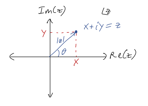
Obviously, numbers along the real axis here are real numbers; numbers on the vertical axis are called imaginary numbers or pure imaginary.
In complete analogy to polar coordinates, we define the magnitude or modulus of \( z \) to be
\[ \begin{aligned} |z| = \sqrt{x^2 + y^2} = \sqrt{{\rm Re}(z)^2 + {\rm Im}(z)^2}. \end{aligned} \]
We can also define an angle \( \theta \), as pictured above, by taking \( \theta = \tan^{-1}(y/x) \) (being careful about quadrants.) This is very useful in a specific context - we'll come back to it in a moment.
First, one more definition: for every \( z = x + iy \), we define the complex conjugate \( z^\star \) to be
\[ \begin{aligned} z^\star = x - iy \end{aligned} \]
(More notation: in math books this is often written \( \bar{z} \) instead of \( z^\star \); physicists tend to prefer the star notation.) In terms of the complex plane, this is a mirror reflection across the \( x \)-axis. We note that
\[ \begin{aligned} zz^\star = (x+iy)(x-iy) = x^2 - i^2 y^2 = x^2 + y^2 \end{aligned} \]
so \( zz^\star = |z|^2 = |z\star|2 \) (the last one is true since \( (z\star)\star = z \).)
Multiplying and dividing complex numbers is best accomplished by doing algebra and using the definition of \( i \). For example,
\[ \begin{aligned} (2+3i)(1-i) = 2 - 2i + 3i - 3i^2 \\ = 5 + i \end{aligned} \]
Division proceeds similarly, except that we should always use the complex conjugate to make the denominator real. For example,
\[ \begin{aligned} \frac{2+i}{3-i} = \frac{2+i}{3-i} \frac{3+i}{3+i} \\ = \frac{6 + 5i + i^2}{9 - i^2} \\ = \frac{6 + 5i - 1}{9 + 1} \\ = \frac{5+5i}{10} = \frac{1}{2} + \frac{i}{2}. \end{aligned} \]
The most important division rule to keep in mind is that dividing by \( i \) just gives an extra minus sign, e.g.
\[ \begin{aligned} \frac{2}{i} = \frac{2i}{i^2} = -2i. \end{aligned} \]
Now, finally to the real reason we're introducing complex numbers: an extremely useful equation called Euler's formula. To find the formula, we start with the series expansion of the exponential function:
\[ \begin{aligned} e^x = 1 + x + \frac{x^2}{2!} + \frac{x^3}{3!} + \frac{x^4}{4!} + ... \end{aligned} \]
Series expansions are just as valid over the complex numbers as over the real numbers (with some caveats, but definitely and always true for the exponential.) What happens if we plug in an imaginary number instead of a real one? Let's try \( x = i\theta \), where \( \theta \) is real:
\[ \begin{aligned} e^{i\theta} = 1 + i\theta + \frac{(i\theta)^2}{2!} + \frac{(i\theta)^3}{3!} + \frac{(i\theta)^4}{4!} + ... \end{aligned} \]
Multiplying out all the factors of \( i \) and rearranging, we find this splits into two series, one with an \( i \) left over and one which is completely real:
\[ \begin{aligned} e^{i\theta} = \left(1 - \frac{\theta^2}{2!} + \frac{\theta^4}{4!} + ... \right) + i \left( \theta - \frac{\theta^3}{3!} + ... \right) \end{aligned} \]
Those other two series should look familiar: they are exactly the Taylor series for the trig functions \( \cos \theta \) and \( \sin \theta \)! With that recognition, we have Euler's formula:
\[ \begin{aligned} e^{i\theta} = \cos \theta + i \sin \theta. \end{aligned} \]
This is an extremely useful and powerful formula, that makes complex numbers much easier to work with! Notice first that
\[ \begin{aligned} |e^{i\theta}| = \cos^2 \theta + \sin^2 \theta = 1. \end{aligned} \]
So \( e^{i\theta} \) is always on the unit circle - and as the notation suggests, the angle \( \theta \) is exactly the angle in the complex plane of this number. This leads to the polar notation for an arbitrary complex number,
\[ \begin{aligned} z = x + iy = |z| e^{i\theta}. \end{aligned} \]
The polar version is much easier to work with for multiplying and dividing complex numbers:
\[ \begin{aligned} z_1 z_2 = |z_1| |z_2| e^{i(\theta_1 + \theta_2)} \\ z_1 / z_2 = |z_1| / |z_2| e^{i(\theta_1 - \theta_2)} \\ z^\alpha = |z|^\alpha e^{i\alpha \theta} \end{aligned} \]
For that last one, we see that taking roots is especially nice in polar coordinates. For example, since \( i = e^{i\pi/2} \), we have
\[ \begin{aligned} \sqrt{i} = e^{i\pi/4} = \frac{1}{\sqrt{2}} (1+i) \end{aligned} \]
which you can easily verify. (This is the principal root, actually; the other possible solution is at \( e^{5i \pi/4} \), which is \( -1 \) times the number above.)
Back to Euler's formula itself: we can invert the formula to find useful equations for \( \cos \) and \( \sin \). I'll leave it as an exercise to prove the following identities:
\[ \begin{aligned} \cos \theta = \frac{1}{2} (e^{i\theta} + e^{-i\theta}) \\ \sin \theta = \frac{-i}{2} (e^{i\theta} - e^{-i\theta}) \end{aligned} \]
(These are, incidentally, extremely useful in simplifying integrals that contain products of trig functions. We'll see this in action later on!)
Complex solutions to the SHO
Back to the SHO equation,
\[ \begin{aligned} \ddot{x} = -\omega^2 x \end{aligned} \]
The minus sign in the equation is very important. We saw before that for equilibrium points that are unstable, the equation of motion we found near the equilibrium was \( \ddot{x} = +\omega^2 x \). This equation has solutions that are exponential in \( t \), moving rapidly away from equilibrium.
But now that we've introduced complex numbers, we can also write an exponential solution to the SHO equation. Notice that if we take \( x(t) = e^{i\omega t} \), then
\[ \begin{aligned} \ddot{x} = \frac{d}{dt} (i \omega e^{i \omega t}) = (i \omega)^2 e^{i \omega t} = -\omega^2 e^{i\omega t} \end{aligned} \]
and so this satisfies the equation. So does the function \( e^{-i\omega t} \) - the extra minus sign cancels when we take two derivatives. These are independent functions, even though they look very similar; there is no constant we can multiply \( e^{i\omega t} \) by to get \( e^{-i \omega t} \). Thus, another way to write the general solution is
\[ \begin{aligned} x(t) = C_1 e^{i\omega t} + C_2 e^{-i \omega t}. \end{aligned} \]
Now, this is a physics class (and we're not doing quantum mechanics!), so obviously the position of our oscillator \( x(t) \) always has to be a real number. However, by introducing \( i \) we have found a solution for \( x(t) \) valid over the complex numbers. The only way that this can make sense is if choosing physical (i.e. real) initial conditions for \( x(0) \) and \( \dot{x}(0) \) gives us an answer that stays real for all time; otherwise, we've made a mistake somewhere.
Let's see how this works by imposing those initial conditions: we have
\[ \begin{aligned} x(0) = x_0 = C_1 + C_2 \\ v(0) = v_0 = i\omega (C_1 - C_2) \end{aligned} \]
This obviously only makes sense if \( C_1 + C_2 \) is real and \( C_1 - C_2 \) is pure imaginary - which means the coefficients \( C_1 \) and \( C_2 \) have to be complex! (This isn't a surprise, since we asked for a solution over complex numbers.) If we write
\[ \begin{aligned} C_1 = x + iy \end{aligned} \]
then the conditions above mean that we must have \( C_2 = x - iy \) so the real and imaginary parts cancel appropriately. In other words, we must have a general solution of the form
\[ \begin{aligned} x(t) = C_1 e^{i\omega t} + C_1^\star e^{-i\omega t}. \end{aligned} \]
This might look confusing, since we now seemingly have one arbitrary constant instead of the two we need. But it's one arbitrary complex number, which is equivalent to two arbitrary reals. In fact, we can finish plugging in our initial conditions to find
\[ \begin{aligned} C_1 = \frac{x_0}{2} - \frac{iv_0}{2\omega} \end{aligned} \]
so both of our initial conditions are indeed separately contained in the single constant \( C_1 \).
Now, if we look at the latest form for \( x(t) \), we notice that the second term is exactly just the complex conjugate of the first term. Recalling the definition of the real part as
\[ \begin{aligned} {\rm Re}(z) = \frac{1}{2} (z + z^\star), \end{aligned} \]
we can rewrite this more compactly as
\[ \begin{aligned} x(t) = 2\ {\rm Re}\ (C_1 e^{i\omega t}). \end{aligned} \]
This is nice, because now \( x(t) \) is manifestly always real! (But remember that we did not just arbitrarily "take the real part" to enforce this; it came out of our initial conditions. It's not correct to solve over the complex numbers and then just ignore half the solution!)
At this point, let's try to compare back to our trig-function solutions; we know they're hiding in there somehow, thanks to Euler's formula.
Exercise - from complex to real
Using \( C_1 \) in terms of \( x_0 \) and \( v_0 \), show that taking the real part of \( C_1 e^{i\omega t} \) gives back our previous general solution,
\[ \begin{aligned} x(t) = x_0 \cos (\omega t) + \frac{v_0}{\omega} \sin (\omega t). \end{aligned} \]
As always, give this a try yourself before you read on!
The best way to do this is to expand our all the complex numbers into real and imaginary components, do some algebra, and then just read off what the real part of the product is. Let's substitute in using both \( C_1 \) from above and Euler's formula:
\[ \begin{aligned} x(t) = 2\ {\rm Re}\ \left[ \left( \frac{x_0}{2} - \frac{iv_0}{2\omega} \right) \left( \cos (\omega t) + i \sin (\omega t) \right) \right] \end{aligned} \]
Pulling the \( 2 \) in from the front and then multiplying through,
\[ \begin{aligned} x(t) = {\rm Re}\ \left[ x_0 \cos(\omega t) + ix_0 \sin (\omega t) - \frac{iv_0}{\omega} \cos (\omega t) + \frac{v_0}{\omega} \sin (\omega t) \right] \\ = {\rm Re}\ \left[ x_0 \cos (\omega t) + \frac{v_0}{\omega} \sin (\omega t) + i (...) \right] \\ = x_0 \cos (\omega t) + \frac{v_0}{\omega} \sin (\omega t) \end{aligned} \]
just ignoring the imaginary part. So indeed, this is exactly the same as our previous solution, just in a different form!
This is a nice confirmation, but the fact that \( C_1 \) is complex makes it a little non-obvious what the real and imaginary parts look like. We can fix that by rewriting it in polar notation. If I suggestively define
\[ \begin{aligned} C_1 = \frac{A}{2} e^{-i\delta}, \end{aligned} \]
then we have
\[ \begin{aligned} x(t) = {\rm Re}\ (A e^{-i\delta} e^{i\omega t}) = A\ {\rm Re}\ (e^{i(\omega t - \delta)}) \end{aligned} \]
pulling the real number \( A \) out of the real part. Now taking the real part of the combined complex exponential is easy: it's just the cosine of the argument,
\[ \begin{aligned} x(t) = A \cos (\omega t - \delta), \end{aligned} \]
exactly matching the other form of the SHO solution we wrote down before. (Notice: no need for trig identities this time! Complex exponentials are a very powerful tool for simplfying expressions involving trig functions.)
I'm going to completely skip over the two-dimensional oscillator; as we emphasized before, one-dimensional motion is special in terms of what we can learn from considering energy conservation, and similarly the SHO is especially useful in one dimension. Of course, the idea of expanding around equilibrium points is very general, but it will not just give you the 2d or 3d SHO equation that Taylor studies in (5.3). In general, you will end up with a coupled harmonic oscillator, the subject of chapter 11.
We can see what happens by just considering the seemingly simple example of a mass on a spring connected to the origin in two dimensions. If the equilibrium (unstretched) length of the spring is \( r_0 \), then
\[ \begin{aligned} \vec{F} = -k(r- r_0) \hat{r} \end{aligned} \]
or expanding in our two coordinates, using \( r = \sqrt{x^2 + y^2} \) and \( \hat{r} = \frac{1}{r} (x\hat{x} + y\hat{y}) \),
\[ \begin{aligned} m \ddot{x} = -kx (1 - \frac{r_0}{\sqrt{x^2 + y^2}}) \\ m \ddot{y} = -ky (1 - \frac{r_0}{\sqrt{x^2 + y^2}}) \end{aligned} \]
These are much more complicated than the regular SHO, and indeed we see they are coupled: both \( x \) and \( y \) appear in both equations. The regular two-dimensional SHO appears when \( r_0 = 0 \), and we just get two nice uncoupled SHO equations; but as I said, this is a special case, so I'll just let you read about it in Taylor.