Last time, we ended by considering an integral of a product of sines,
\[ \begin{aligned} \int_{-\tau/2}^{\tau/2} \sin(3 \omega t) \sin(5 \omega t) dt = ? \end{aligned} \]
We could painstakingly apply trig identities to break this down into a number of integrals over \( \sin(\omega t) \) and \( \cos (\omega t) \). However, a much better way to approach this problem is using complex exponentials. Let's try this related complex-exponential integral first:
\[ \begin{aligned} \int_{-\tau/2}^{\tau/2} e^{3i\omega t} e^{5i \omega t} dt = \int_{-\tau/2}^{\tau/2} e^{8i \omega t} dt \\ = \left. \frac{1}{8i \omega} e^{8i \omega t} \right|_{-\tau/2}^{\tau/2} \\ = \frac{1}{8i \omega} \left[ e^{4i \omega \tau} - e^{-4i \omega \tau} \right] = 0 \end{aligned} \]
where as in our original example, we know that the complex exponentials are periodic, \( e^{i\omega (t + n\tau)} = e^{i \omega t} \), so the terms in square brackets cancel off. No trig identities needed here!
Let's do the fully general case for complex exponentials, to see whether there's anything special about the numbers we've chosen here.
\[ \begin{aligned} \int_{-\tau/2}^{\tau/2} e^{im\omega t} e^{in \omega t} dt = \int_{-\tau/2}^{\tau/2} e^{i(m+n)\omega t} dt \\ = \left. \frac{1}{(m+n)i \omega} e^{i(m+n)\omega t} \right|_{-\tau/2}^{\tau/2} \\ = \frac{1}{(m+n)i \omega} \left[ e^{i(m+n) \omega \tau/2} - e^{-i(m+n) \omega \tau/2} \right] \\ = \frac{1}{(m+n) i \omega} e^{i(m+n) \omega \tau} \left[1 - e^{-2\pi i(m+n)} \right], \end{aligned} \]
using \( \omega \tau = 2\pi \) on the last line. This is always zero, as long as \( m \) and \( n \) are both integers, since \( e^{2\pi i} \) is just 1. However, there is an edge case we ignored: if \( m = -n \), then we have a division by zero. This is because we didn't do the integral correctly in that special case:
\[ \begin{aligned} \int_{-\tau/2}^{\tau/2} e^{-in \omega t} e^{in \omega t} dt = \int_{-\tau/2}^{\tau/2} dt = \tau. \end{aligned} \]
We can write this result compactly using the following notation:
\[ \begin{aligned} \frac{1}{\tau} \int_{-\tau/2}^{\tau/2} e^{-im \omega t} e^{in \omega t} dt = \delta_{mn} \end{aligned} \]
where \( \delta_{mn} \) is a special symbol called the Kronecker delta symbol, and it means the following:
\[ \begin{aligned} \delta_{mn} = \begin{cases} 1, & m = n; \\ 0, & m \neq n. \end{cases} \end{aligned} \]
In other words, the integral over a single period of two complex exponential functions \( e^{in\omega t} \) is always zero unless they have equal and opposite values of \( n \) and cancel off under the integral.
Now we're ready to go back to the related integral that we started with, over products of sines and cosines. We can rewrite it using complex exponentials to apply our results:
\[ \begin{aligned} \int_{-\tau/2}^{\tau/2} \sin(3 \omega t) \sin(5 \omega t) dt = \int_{-\tau/2}^{\tau/2} \frac{1}{2i} \left( e^{3i\omega t} - e^{-3i\omega t}\right) \frac{1}{2i} \left( e^{5i \omega t} - e^{-5i \omega t} \right) dt \\ = -\frac{1}{4} \int_{-\tau/2}^{\tau/2} \left( e^{8i \omega t} - e^{-2i\omega t} - e^{2i \omega t} + e^{-8i \omega t} \right) dt \\ = 0, \end{aligned} \]
since none of the pairs of complex exponential terms cancel each other off. In fact, we can easily extend this to the general case:
\[ \begin{aligned} \int_{-\tau/2}^{\tau/2} \sin(m \omega t) \sin(n \omega t) dt = -\frac{1}{4} \int_{-\tau/2}^{\tau/2} \left( e^{im\omega t} - e^{-im \omega t} \right) \left( e^{in \omega t} - e^{-in \omega t} \right) dt \\ = -\frac{1}{4} \int_{-\tau/2}^{\tau/2} \left( e^{i(m+n)\omega t} + e^{-i(m+n) \omega t} - e^{i(m-n) \omega t} - e^{-i(m-n) \omega t}\right) dt \end{aligned} \]
Assuming \( m \) and \( n \) are both positive, the only way this will ever give a non-zero answer is if \( m=n \), in which case we have
\[ \begin{aligned} -\frac{1}{4} \int_{-\tau/2}^{\tau/2} (-2 dt) = \frac{\tau}{2}. \end{aligned} \]
(If we had a negative \( m \) or \( n \), we could use a trig identity to rewrite it, i.e. \( \sin(-m\omega t) = -\sin(m \omega t) \).) Again using the Kronecker delta symbol to write this compactly, we have the important result
\[ \begin{aligned} \frac{2}{\tau} \int_{-\tau/2}^{\tau/2} \sin (m \omega t) \sin (n \omega t) dt = \delta_{mn}. \end{aligned} \]
It's not difficult to show that similarly,
\[ \begin{aligned} \frac{2}{\tau} \int_{-\tau/2}^{\tau/2} \cos (m \omega t) \cos (n \omega t) dt = \delta_{mn}, \\ \frac{2}{\tau} \int_{-\tau/2}^{\tau/2} \sin (m \omega t) \cos (n \omega t) dt = 0, \end{aligned} \]
again for positive \( (>0) \) integer values of \( m \) and \( n \). (This last formula is obvious, even without going into complex exponentials: this is the integral of an odd function times an even function over a symmetric interval, so it must be zero.)
The combination of these three results is incredibly powerful when applied to a Fourier series! Recall that the definition of the Fourier series representation of a function \( f(t) \) was
\[ \begin{aligned} f(t) = \sum_{n=0}^\infty \left[ a_n \cos(n \omega t) + b_n \sin (n \omega t) \right]. \end{aligned} \]
Suppose we want to know what the coefficient \( a_4 \) is. Thanks to the integral formulas we found above, if we integrate the entire series against the function \( \cos(4 \omega t) \), the integral will vanish for every term except precisely the one we want:
\[ \begin{aligned} \frac{2}{\tau} \int_{-\tau/2}^{\tau/2} f(t) \cos(4 \omega t) dt \\ = \frac{2}{\tau} \sum_{n=0}^\infty \left[ a_n \int_{-\tau/2}^{\tau/2} \cos (n \omega t) \cos (4 \omega t) dt + b_n \int_{-\tau/2}^{\tau/2} \sin(n \omega t) \cos (4 \omega t) dt \right] \\ = \sum_{n=0}^{\infty} \left[ a_n \delta_{n4} + b_n (0) \right] = a_4. \end{aligned} \]
In fact, we can now write down a general integral formula for all of the coefficients in the Fourier series:
\[ \begin{aligned} a_n = \frac{2}{\tau} \int_{-\tau/2}^{\tau/2} f(t) \cos(n \omega t) dt, \\ b_n = \frac{2}{\tau} \int_{-\tau/2}^{\tau/2} f(t) \sin(n \omega t) dt, \\ a_0 = \frac{1}{\tau} \int_{-\tau/2}^{\tau/2} f(t) dt, \\ b_0 = 0. \end{aligned} \]
The \( n=0 \) cases are special, and I've split them out: of course, \( b_0 \) is always multiplying the function \( \sin(0) = 0 \), so it doesn't matter what it is - we can just ignore it. As for \( a_0 \), it is a valid part of the Fourier series, but it corresponds to a constant offset. We find its value by just integrating the function \( f(t) \); this integral is zero for any of the trig functions, but just gives back \( \tau \) on the constant \( a_0 \) term.
Let's take a moment to appreciate the power of this result! To calculate a Taylor series expansion of a function, we have to compute derivatives of the function over and over until we reach the desired truncation order. These derivatives will generally become more and more complicated to deal with as they generate more terms with each iteration. On the other hand, for the Fourier series we have a direct and simple formula for any coefficient; finding \( a_{100} \) is no more difficult than finding \( a_1 \)! So the Fourier series is significantly easier to extend to very high order.
A useful analogy: Fourier series and vector spaces
Before we do an example, a few more important thoughts on those crucial integral identities that let us pick off the Fourier series coefficients. Actually, I want to start with the new symbol we introduced, the Kronecker delta symbol. We actually could have introduced this symbol all the way back at the beginning of the semester, when we were talking about vector coordinates. Remember that for a general three-dimensional coordinate system, we can expand any vector in terms of three unit vectors:
\[ \begin{aligned} \vec{a} = a_1 \hat{e}_1 + a_2 \hat{e}_2 + a_3 \hat{e}_3. \end{aligned} \]
The dot product of any two vectors is given by multiplying the components for each unit vector in turn:
\[ \begin{aligned} \vec{a} \cdot \vec{b} = (a_1 \hat{e}_1 + a_2 \hat{e}_2 + a_3 \hat{e}_3) \cdot (b_1 \hat{e}_1 + b_2 \hat{e}_2 + b_3 \hat{e}_3) \\ = a_1 b_1 + a_2 b_2 + a_3 b_3. \end{aligned} \]
What if we just take dot products of the unit vectors themselves, so \( a_i \) and \( b_i \) are either 1 or 0? We immediately see that we'll get 1 for the dot product of any unit vector with itself, and 0 otherwise, for example
\[ \begin{aligned} \hat{e}_1 \cdot \hat{e}_1 = 1, \\ \hat{e}_1 \cdot \hat{e}_3 = 0, \end{aligned} \]
and so on. The compact way to write this relationship is using the Kronecker delta again:
\[ \begin{aligned} \hat{e}_i \cdot \hat{e}_j = \delta_{ij}. \end{aligned} \]
This leads us to a technical math term that I didn't introduce before: the set of unit vectors \( {\hat{e}_1, \hat{e}_2, \hat{e}_3} \) form an orthonormal basis. "Basis" here means that we can write any vector at all as a combination of the unit vectors. Orthonormal means that all of the unit vectors are mutually perpendicular, and they all have length 1. Saying that the dot products of the unit vectors is given by the Kronecker delta is the same thing as saying they are orthonormal! Orthonormality is a useful property because it's what allows us to write the dot product in the simplest way possible.
Now let's imagine a fictitious space that has more than 3 directions, let's say some arbitrary number \( N \). We can use the same language of unit vectors to describe that space, and once again, it's most convenient to work with an orthonormal basis. It's really easy to extend what we've written above to this case! We find a set of vectors \( {\hat{e}_1, \hat{e}_2, ..., \hat{e}_N} \) that form a basis, and then ensure that they are orthonormal, which is still written in exactly the same way,
\[ \begin{aligned} \hat{e}_i \cdot \hat{e}_j = \delta_{ij}. \end{aligned} \]
We can then expand an arbitrary vector out in terms of unit-vector components,
\[ \begin{aligned} \vec{a} = a_1 \hat{e}_1 + a_2 \hat{e}_2 + ... + a_N \hat{e}_N. \end{aligned} \]
Larger vector spaces like this turn out to be very useful, even for describing the real world. You'll have to wait until next semester to see it, but they show up naturally in describing systems of physical objects, for example a set of three masses all joined together with springs. Since each individual object has three coordinates, it's easy to end up with many more than 3 coordinates to describe the entire system at once.
Let's wrap up the detour and come back to our current subject of discussion, which is Fourier series. This example is partly meant to help you think about the Kronecker delta symbol, but the analogy between Fourier series and vector spaces actually goes much further than that. Recall the definition of a (truncated) Fourier series is
\[ \begin{aligned} f_M(t) = a_0 + \sum_{n=1}^M \left[a_n \cos (n \omega t) + b_n \sin (n \omega t) \right]. \end{aligned} \]
Expanding the function \( f(t) \) out in terms of a set of numerical coefficients \( {a_n, b_n} \) strongly resembles what we do in a vector space, expanding a vector out in terms of its vector components. We can think of rewriting the Fourier series in vector-space language,
\[ \begin{aligned} f_M(t) = a_0 \hat{e}_0 + \sum_{n=1}^M \left[ a_n \hat{e}_n + b_n \hat{e}_{M+n} \right] \end{aligned} \]
defining a set of \( 2M-1 \) "unit vectors",
\[ \begin{aligned} \hat{e}_0 = 1, \\ \hat{e}_{n} = \begin{cases} \cos(n \omega t),& 1 \leq n \leq M; \\ \sin(n \omega t),& M+1 \leq n \leq 2M; \end{cases} \end{aligned} \]
As you might suspect, the "dot product" (more generally known as an inner product) for this "vector space" is defined by doing the appropriate integral for the product of unit functions:
\[ \begin{aligned} \hat{e}_m \cdot \hat{e}_n = \frac{2}{\tau} \int_{-\tau/2}^{\tau/2} (\hat{e}_m) (\hat{e}_n) dt = \delta_{mn}. \end{aligned} \]
So our "unit vectors" are all orthonormal, and the claim that we can do this for any function \( f(t) \) means that they form an orthonormal basis!
I should emphasize that the space of functions is not really a vector space - mathematically, there are important differences. But there are enough similarities that this is a very useful analogy for conceptually thinking about what a Fourier series means. Just like a regular vector space, the Fourier series decomposition is nothing more than expanding the "components" of a periodic function in terms of the orthonormal basis given by \( \cos(n\omega t) \) and \( \sin(n \omega t) \). (Unlike a regular vector space, and more like a Taylor series, the contributions from larger \( n \) tend to be less important, so we can truncate the series and still get a reasonable answer. In a regular vector space, there's no similar reason to truncate our vectors!)
Example: the sawtooth wave
Let's do a concrete and simple example of a Fourier series decomposition. Consider the following function which is periodic but always linearly increasing (this is sometimes called the sawtooth wave):
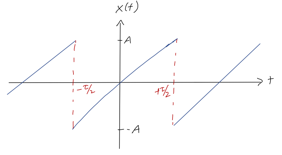
The equation describing this curve is
\[ \begin{aligned} x(t) = 2A\frac{t}{\tau},\ -\frac{\tau}{2} \leq t < \frac{\tau}{2} \end{aligned} \]
Next time, we'll continue this example.