Last time, we set up the sawtooth wave as an example of a periodic function:
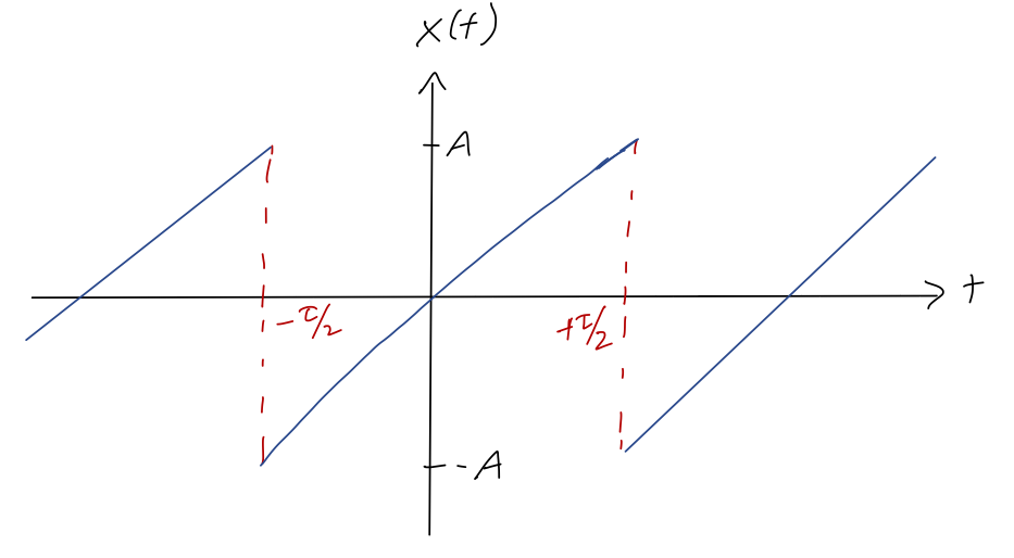
The equation describing this curve is
\[ \begin{aligned} x(t) = 2A\frac{t}{\tau},\ -\frac{\tau}{2} \leq t < \frac{\tau}{2} \end{aligned} \]
Let's find the Fourier series coefficients for this curve. We'll begin with the simplest integral, for \( a_0 \):
\[ \begin{aligned} a_0 = \frac{1}{\tau} \int_{-\tau/2}^{\tau/2} x(t) dt = \frac{1}{\tau} \int_{-\tau/2}^{\tau/2} \frac{2A}{\tau} t\ dt \end{aligned} \]
We can stop right here, because the function \( t \) is odd, and we're doing an integral which is symmetric around the origin, so the integral has to vanish: \( a_0 = 0 \). (Again, the argument is that the odd symmetry means that the two parts of the integral from \( -\tau/2 \) to \( 0 \) and from \( 0 \) to \( +\tau/2 \) are equal and opposite; this should be easy to see from the plot above!)
In fact, this argument extends to all of the \( a_n \) coefficients: writing the integral out,
\[ \begin{aligned} a_n = \frac{4A}{\tau^2} \int_{-\tau/2}^{\tau/2} t \cos(n \omega t) dt = 0 \end{aligned} \]
since the combination of even \( \cos \) and odd \( t \) in the integral is again an odd function. Thus, the only non-zero Fourier coefficients will be the \( b_n \). In fact, this is something we should always look for when computing Fourier series: if the function to be expanded is odd, then all of the \( a_n \) will vanish (including \( a_0 \)), whereas if it is even, all the \( b_n \) will vanish instead.
On to the integrals we actually have to compute:
\[ \begin{aligned} b_n = \frac{4A}{\tau^2} \int_{-\tau/2}^{\tau/2} t \sin(n \omega t) dt \end{aligned} \]
This is a great candidate for integration by parts. Rewriting the integral as \( \int u dv \), we have
\[ \begin{aligned} u = t \Rightarrow du = dt \\ dv = \sin (n \omega t) dt \Rightarrow v = -\frac{1}{n \omega} \cos (n \omega t) \end{aligned} \]
and so
\[ \begin{aligned} \int u\ dv = uv - \int v\ du \\ = \left. -\frac{1}{n \omega} t \cos (n \omega t) \right|_{-\tau/2}^{\tau/2} + \frac{1}{n \omega} \int_{-\tau/2}^{\tau/2} \cos(n \omega t) dt \\ = -\frac{1}{n \omega} \left[ \frac{\tau}{2} \cos (n\pi) - \frac{-\tau}{2} \cos (-n\pi) \right] + \frac{1}{n^2 \omega^2} \left[ \sin (n \pi) - \sin (-n\pi) \right] \end{aligned} \]
The second term just vanishes since \( \sin(n\pi) = 0 \) for any integer \( n \). As for the first term, \( \cos(n\pi) \) is either \( +1 \) if \( n \) is even, or \( -1 \) if \( n \) is odd. Since \( \cos(-n\pi) = \cos(n\pi) \), we have the overall result
\[ \begin{aligned} \int u\ dv = -\frac{1}{n\omega} \left[ \frac{\tau}{2} (-1)^n + \frac{\tau}{2} (-1)^n \right] = -\frac{\tau}{n \omega} (-1)^n, \end{aligned} \]
or plugging the integral back into the Fourier coefficient formula,
\[ \begin{aligned} b_n = \frac{4A}{\tau^2} \int u\ dv = \frac{-4A \tau}{n \omega \tau^2} (-1)^n = -\frac{2A}{\pi n} (-1)^n = \frac{2A}{\pi n} (-1)^{n+1}, \end{aligned} \]
absorbing the overall minus sign at the very end. And now we're done - we have the entire Fourier series, all coefficients up to arbitrary \( n \) as a simple formula! Once again, you can appreciate how much easier it is to keep many terms before truncating in this case, compared to using a Taylor series. Plugging in some numbers to get a feel for this, the first few coefficients are
\[ \begin{aligned} b_1 = \frac{2A}{\pi},\ b_2 = -\frac{A}{\pi}, b_3 = \frac{2A}{3\pi}, b_4 = -\frac{A}{2\pi}, ... \end{aligned} \]
Importantly, the size of the coefficients is shrinking as \( n \) increases, due to the \( 1/n \) in our formula. Unlike the Taylor series, there is no automatic factor of \( 1/n! \) to help with convergence, so we should worry a little about the accuracy of truncating a Fourier series! It is, nevertheless, quite generic for the size of the Fourier series coefficients to die off in some way with \( n \). Remember that we're building a function up out of sines and cosines. Functions like \( \cos(n \omega t) \) with \( n \) very large are oscillating very, very quickly; if the function we're building up is relatively smooth, it makes sense that the really fast-oscillating terms won't be very important in modeling it.
Let's plug in some numbers and get a feel for how well our Fourier series does in approximating the sawtooth wave! Choosing \( A=1 \) and \( \omega = 2\pi \) (so \( \tau = 1 \)), here are some plots keeping the first \( m \) terms before truncating:
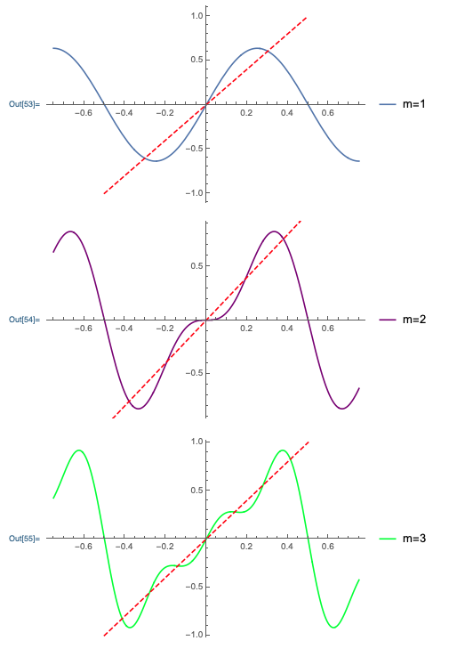
We can see that even as we add the first couple of terms, the approximation of the Fourier series curve to the sawtooth (the red line, plotted just for the region from \( -\tau/2 \) to \( \tau/2 \)) is already improving rapidly.
To visualize a bit better what's happening here, let's look at the three separate components of the final \( m=3 \) curve:
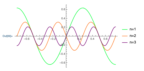
We clearly see that the higher-\( n \) components are getting smaller. If you compare the two plots, you can imagine "building up" the linear sawtooth curve one sine wave at a time, making finer adjustments at each step.
Of course, although \( m=3 \) might be closer to the sawtooth than you expected, it's still not that great - particularly near the edges of the region. Since we have an analytic formula, let's jump to a nice high truncation of \( m=50 \):
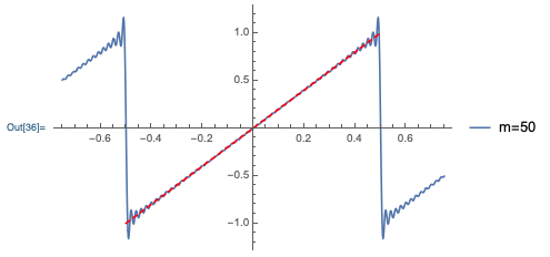
This is a remarkably good approximation - it's difficult to see the difference between the Fourier series and the true curve near the middle of the plot! At the discontinuities at \( \pm \tau/2 \), things don't work quite as well; we see the oscillation more clearly, and the Fourier series is overshooting the true amplitude by a bit. In fact, this effect (known as the Gibbs phenomenon) persists no matter how many terms we keep: there is a true asymptotic (\( n \rightarrow \infty \)) error in the Fourier series approximation whenever our function jumps discontinuously, so we never converge to exactly the right function.
The good news is that as we add more terms, this overshoot gets arbitrarily close to the discontinuity (the Gibbs phenomenon gets narrower), so we can still improve our approximation in that way. We'll always be stuck with this effect at the discontinuity, but of course real-world functions don't really have discontinuities, so this isn't really a problem in practice.
We could try to look at a plot of all of the 50 different sine waves that build up the \( m=50 \) sawtooth wave above, but it would be impossible to learn anything from the plot because it would be too crowded. Instead of looking at the whole sine waves, a different way to visualize the contributions is just to plot the coefficients \( |b_n| \) vs. \( n \):
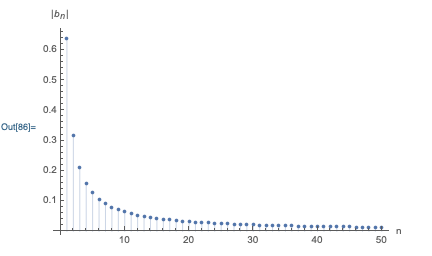
The qualitative \( 1/n \) behavior of the coefficients is immediately visible. This plot is sometimes known as a frequency domain plot, because the \( n \) on the horizontal axis is really a label for the size of the sine-function components with frequency \( n\omega \). If we didn't have a simple analytic formula and had to do the integrals for the \( a_n \) and \( b_n \) numerically, such a plot gives a simple way to check at a glance that the Fourier series is converging.
At this point I'll go back to the physics, but have a look in Taylor for a second example of finding the Fourier coefficients of a simple periodic function.
Solving the damped, driven oscillator with Fourier series
Now we're ready to come back to our physics problem: the damped, driven oscillator. Suppose now that we have a totally arbitrary driving force \( F(t) \), which is periodic with period \( \tau \):
\[ \begin{aligned} \ddot{x} + 2\beta \dot{x} + \omega_0^2 x = \frac{F(t)}{m} \end{aligned} \]
Since \( F(t) \) is periodic, we can find a Fourier series decomposition:
\[ \begin{aligned} F(t) = \sum_{n=0}^\infty \left[ a_n \cos (n \omega t) + b_n \sin (n \omega t) \right] \end{aligned} \]
As we saw before, if the driving force consists of multiple terms, we can just solve for one particular solution at a time and add them together. So in fact, we know exactly how to solve this already! The particular solution has to be
\[ \begin{aligned} x_p(t) = \sum_{n=0}^\infty \left[ A_n \cos (n \omega t - \delta_n) + B_n \sin (n \omega t - \delta_n) \right] \end{aligned} \]
where the amplitudes and phase shifts for each term are exactly what we found before, just using \( n \omega \) as the driving frequency:
\[ \begin{aligned} A_n = \frac{a_n/m}{\sqrt{(\omega_0^2 - n^2\omega^2)^2 + 4\beta^2 n^2 \omega^2}} \\ B_n = \frac{b_n/m}{\sqrt{(\omega_0^2 - n^2\omega^2)^2 + 4\beta^2 n^2 \omega^2}} \\ \delta_n = \tan^{-1} \left( \frac{2\beta n \omega}{\omega_0^2 - n^2 \omega^2} \right) \end{aligned} \]
At long times, this is the full solution: at short times, we add in the transient terms due to the complementary solution. (Note that the special case \( n=0 \), corresponding to a constant driving piece \( F_0 \), doesn't require a different formula - it's covered by the ones above, as you can check!)
So at the minor cost of finding a Fourier series for the driving force, we can immediately write down the solution for the corresponding driven, damped oscillator! There are a couple of additional points that are worth making here:
First, remember that the energy of a simple harmonic oscillator is just \( E = \frac{1}{2} kA^2 \). At long times, when the system reaches its steady state, the Fourier decomposition tells us that it is nothing more than a combination of lots of simple harmonic oscillators! Thus, we can easily find the total energy by just adding up all of the individual contributions.
Second, everything we said about resonance remains true for this more general case of a driving force. The key difference is that while our object still has a single natural frequency \( \omega_0 \), we now have multiple driving frequencies \( \omega, 2\omega, 3\omega... \) all active at once! As a result, if we drive at a low frequency \( \omega \ll \omega_0 \), we can still encounter resonance as long as \( n\omega \approx \omega_0 \) for some integer value \( n \). This effect is balanced by the fact that the amplitude of the higher modes is dying off as \( n \) increases, but since the effect of resonance is so dramatic, we'll still see some effect from the higher mode being close to \( \omega_0 \).
(A simple everyday example of this effect is a playground swing, which typically has a natural frequency of roughly \( \omega_0 \sim 1 \) Hz. If you are pushing a child on a swing, and you try to push at a higher frequency than \( \omega_0 \), you won't be very successful - all of the modes of your driving force are larger than \( \omega_0 \), so no resonance. On the other hand, pushing less frequently can still work, as long as \( n \omega \sim \omega_0 \), e.g. pushing them once every 3 or 4 seconds will still lead to some amount of resonance.)
Let's see how this works by putting our previous example to work.
Example: sawtooth driving force
Suppose we have a driving force which is described well by a sawtooth wave, the same function that we found the Fourier series for above:
\[ \begin{aligned} F(t) = 2F_0 \frac{t}{\tau},\ -\frac{\tau}{2} \leq t \leq \frac{\tau}{2}. \end{aligned} \]
What is the response of a damped, driven oscillator to this force?
Our starting point is finding the Fourier series to describe \( F(t) \), but we already did that: we know that \( a_n = 0 \) and
\[ \begin{aligned} b_n = \frac{2F_0}{\pi n} (-1)^{n+1}. \end{aligned} \]
Thus, applying our solution for the damped driven oscillator, we have for the particular solution
\[ \begin{aligned} x_p(t) = \sum_{n=0}^\infty B_n \sin(n \omega t - \delta_n) \end{aligned} \]
where
\[ \begin{aligned} B_n = \frac{2(-1)^{n+1} F_0/m}{\pi n\sqrt{(\omega_0^2 - n^2 \omega^2)^2 + 4\beta^2 n^2 \omega^2}}, \\ \delta_n = \tan^{-1} \left( \frac{2\beta n\omega}{\omega_0^2 - n^2 \omega^2} \right). \end{aligned} \]
If we want the full solution, we add in whatever the corresponding particular solution is. For example, if the system is underdamped (\( \beta < \omega_0 \)), then
\[ \begin{aligned} x(t) = A e^{-\beta t} \cos (\sqrt{\omega_0^2 - \beta^2} t - \delta) + x_p(t) \end{aligned} \]
with \( A \) and \( \delta \) determined by our initial conditions. This solution is nice and easy to write down, but very difficult to work with by hand, particularly if we want to keep more than the first couple of terms in the Fourier series! T