Let's continue our study of the following periodic force, which resembles a repeated impulse force:
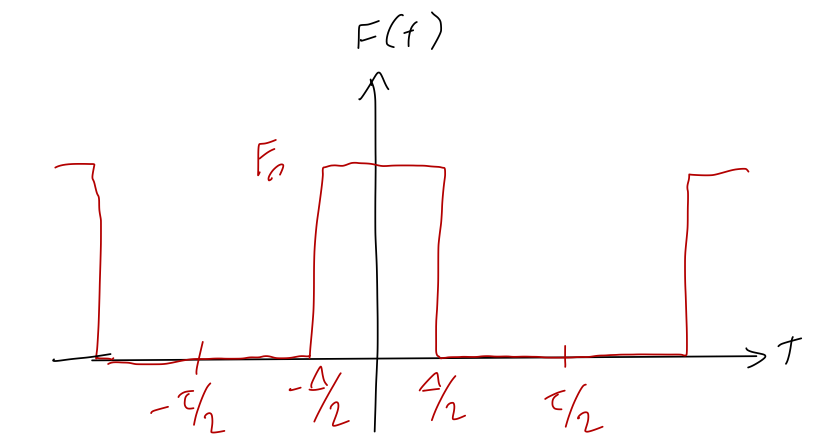
Within the repeating interval from \( -\tau/2 \) to \( \tau/2 \), we have a much shorter interval of constant force extending from \( -\Delta/2 \) to \( \Delta/2 \). It's straightforward to find the Fourier series for this force, but we don't have to because Taylor already worked it out as his example 5.4; the result is
\[ \begin{aligned} a_0 = \frac{F_0 \Delta}{\tau}, \\ a_n = \frac{2F_0}{n\pi} \sin \left( \frac{\pi n \Delta}{\tau} \right), \end{aligned} \]
and all of the \( b_n \) coefficients are zero by symmetry, since the force is even.
Now, to apply this to the single impulse, we want to take the limit where \( \tau \gg \Delta \). This is straightforward to do in the Fourier coefficients themselves: we have
\[ \begin{aligned} a_n \approx \frac{2F_0 \Delta}{\tau}. \end{aligned} \]
But now we run into a problem when we try to actually use the Fourier series, which takes the approximate form
\[ \begin{aligned} F(t) \approx \frac{F_0 \Delta}{\tau} \left[1 + 2 \sum_{n=1}^\infty \cos \left( \frac{2\pi n t}{\tau} \right) \right]. \end{aligned} \]
The problem is that the usual factor of \( 1/n \) cancelled out, so the size of our terms is not dying off as \( n \) increases. So our usual approach of truncation won't be useful at all!
There's something else that is happening at the same time as we try to take \( \tau \rightarrow \infty \), which is equivalent to \( \omega \rightarrow 0 \). Remember that we're summing up distinct Fourier components with frequency \( \omega, 2\omega, 3\omega... \) But as \( \omega \) goes to zero, these frequencies are getting closer and closer together - and our sum is getting closer and closer to resembling a continuous integral!
This suggests that we try to replace the sum with an integral. We want to think carefully about the limit that \( \tau \rightarrow \infty \). Let's define the quantity
\[ \begin{aligned} \omega_n = \frac{2\pi n}{\tau}. \end{aligned} \]
As \( \tau \) becomes larger and larger, the interval between \( \omega_n \) is becoming smaller and smaller, to the point that we can imagine it becoming an infinitesmal:
\[ \begin{aligned} d\omega = \frac{2\pi}{\tau} \Delta n \end{aligned} \]
where \( (\Delta n) = 1 \) by definition, since we sum over integers, but it will be useful notation for what comes next. Let's take this and rewrite the Fourier sum slightly:
\[ \begin{aligned} F(t) = \sum_{n=0}^\infty (\tau a_n) \cos \left( \omega_n t \right) \frac{\Delta n}{\tau} \end{aligned} \]
All I've done is multiplied by 1 twice: first to introduce \( \Delta n \), which is 1, and second to multiply and divide by \( \tau \). But the key is that this is now a sum over a bunch of steps which are infinitesmally small, so as \( \tau \rightarrow \infty \), this is a proper Riemann sum and it becomes an integral. Using \( \Delta n / \tau = d\omega / (2\pi) \), we can write it as an integral over \( \omega \):
\[ \begin{aligned} F(t) = \frac{1}{2\pi} \int_0^\infty G(\omega) \cos(\omega t) d\omega. \end{aligned} \]
The function \( G(\omega) \) comes from the Fourier coefficients, specifically from the product \( \tau a_n \):
\[ \begin{aligned} G(\omega) = \lim_{\tau \rightarrow \infty} \tau \left( \frac{2}{\tau} \int_{-\tau/2}^{\tau/2} f(t) \cos \left( \omega t \right) dt \right) \\ = 2 \int_{-\infty}^\infty f(t) \cos(\omega t) dt. \end{aligned} \]
The function \( G(\omega) \) is known as the Fourier transform of \( F(t) \). Once again, just like the Fourier series, this is a representation of the function. In this case, there's no questions about infinite series or truncation; we're trading one function \( F(t) \) for another function \( G(\omega) \). There is also no restriction about periodicity - we can use the Fourier transform for any function at all, periodic or not.
One note: there are several equivalent but slightly different-looking ways to define the Fourier transform! One simple difference to watch out for is where the factor of \( 2\pi \) goes - it can be partly or totally moved into the definition of \( G(\omega) \) instead of being kept in \( F(t) \). More importantly, the cosine version that we're using is actually not as commonly used, in part because it can only work on functions that are even; in general we need both sine and cosine. A more common definition of the Fourier transform is in terms of complex exponentials:
\[ \begin{aligned} F(t) = \int_{-\infty}^\infty G(\omega) e^{i\omega t} d\omega \\ G(\omega) = \frac{1}{2\pi} \int_{-\infty}^\infty F(t) e^{-i\omega t} dt. \end{aligned} \]
Notice that in this case, unlike the Fourier series, there's a certain symmetry to the definitions of \( F(t) \) and \( G(\omega) \). This is because both representations are functions here, instead of trying to match a function onto a sum. But the symmetry of the definitions suggests that it should be just as good to go backwards, thinking of \( F(t) \) as a representation obtained from \( G(\omega) \).
The Dirac delta function
To understand inverting the Fourier transform, we can take these formulas and plug them in to each other. Let's use the complex exponential version:
\[ \begin{aligned} G(\omega) = \frac{1}{2\pi} \int_{-\infty}^\infty \left( \int_{-\infty}^\infty G(\alpha) e^{i\alpha t} d\alpha \right) e^{-i \omega t} dt \end{aligned} \]
(notice that I can't use \( \omega \) twice. In the definition of \( F(t) \), \( \omega \) is a dummy variable; we're integrating over it, so I can call it anything I want.) Now, I can do some rearranging of these integrals:
\[ \begin{aligned} G(\omega) = \int_{-\infty}^\infty G(\alpha) \left[ \frac{1}{2\pi} \int_{-\infty}^\infty e^{i(\alpha-\omega)t} dt \right] d\alpha \end{aligned} \]
Notice what is going on here; we have the same function \( G \) on both sides of the equation, but on the left it's at a single frequency \( \omega \), while on the right it's integrated over all possible frequencies. This is sort of familiar, actually; it resembles the orthogonality relation we had for the cosines and sines in the Fourier series, where the integral would be zero except for the special case where the two cosines match in frequency.
In line with the idea of orthogonality, the only way this equation can be true for all \( \omega \) and all \( G \) is if the object in square brackets is picking out only \( \alpha = \omega \) from under the integral, and discarding everything else! In other words, if we define
\[ \begin{aligned} \delta(\alpha - \omega) \equiv \frac{1}{2\pi} \int_{-\infty}^\infty e^{i(\alpha - \omega) t} dt, \end{aligned} \]
known as the Dirac delta function (although technically it's not a function - more on that shortly), then it has the property that
\[ \begin{aligned} \int_{-\infty}^\infty dx f(x) \delta(x-a) = f(a). \end{aligned} \]
The delta function resembles the Kronecker delta symbol, in that it "picks out" a certain value of \( x \) from an integral, which is what the Kronecker delta does to a sum. Note that we can put in any function we want, so if we use \( f(x) = 1 \), we get the identity
\[ \begin{aligned} \int_{-\infty}^\infty dx \delta(x) = 1. \end{aligned} \]
In other words, if we think of \( \delta(x) \) as a function on its own, the "area under the curve" is equal to 1. At the same time, we know that it is picking off a very specific value of \( x \) from any given function. Combining these two properties, if we try to plot \( \delta(x) \), it must look something like this:
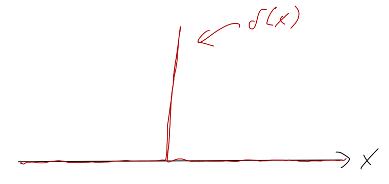
or defining it as a "function",
\[ \begin{aligned} \delta(x) = \begin{cases} \infty, & x = 0; \\ 0, & x \neq 0. \end{cases} \end{aligned} \]
such that the integral over \( \delta(x) \) gives 1, as we found above. Once again, this isn't technically a function, so it's a little dangerous to try to interpret it unless it's safely inside of an integral. (If you're worried about mathematical rigor, it is possible to define the delta function as a limit of a regular function, for example a Gaussian curve, as its width goes to zero.)
From the plot, we can visually observe that it's important that the delta function spike is located within the integration limits, or else we won't pick it up and will just end up with zero. In other words,
\[ \begin{aligned} \int_{-1}^3 dx\ \delta(x-1) = 1 \end{aligned} \]
but
\[ \begin{aligned} \int_{-1}^3 dx\ \delta(x-4) = 0. \end{aligned} \]
There are some other useful properties of the delta function that we could derive (you can look them up in a number of math references, including on Wikipedia or Mathworld.) Let's prove a simple one, to get used to delta-function manipulations a bit. What is \( \delta(kt) \), where \( k \) is a constant real number? As always, to make sense of this we really need to put it under an integral:
\[ \begin{aligned} \int_{-\infty}^\infty f(t) \delta(kt) dt = ? \end{aligned} \]
We can do a simple \( u \)-substitution to rewrite:
\[ \begin{aligned} (...) = \int_{t=-\infty}^{t=\infty} f\left(\frac{u}{k} \right) \delta(u) \frac{du}{k} \\ = \frac{1}{k} \int_{-\infty}^\infty f\left( \frac{u}{k} \right) \delta(u) du \end{aligned} \]
assuming \( k>0 \) for the moment; we'll come back to the possibility of negative \( k \) shortly. Now, the fact that the argument of \( f \) has a \( 1/k \) in it doesn't matter, because when we do the integral we pick off \( f(0) \):
\[ \begin{aligned} (...) = \frac{f(0)}{k} = \int_{-\infty}^\infty f(t) \left[ \frac{1}{k} \delta(t) \right] dt. \end{aligned} \]
Now compare what we started with and what we ended with, and we get \( \delta(kt) = \delta(t)/k \). Again, if \( k<0 \) we get an extra sign flip, which would give us a minus sign - but \( -k \) if \( k \) is negative is just \( |k| \). So we have the full result
\[ \begin{aligned} \delta(kt) = \frac{1}{|k|} \delta(t). \end{aligned} \]
One more comment on the delta function, bringing us back towards physics. We use the delta function often to represent "point particles", which we imagine as being concentrated at a single point in space - not totally realistic, but often a useful approximation. In fact, one example where this is realistic is if we want to describe the charge density of a fundamental charge like an electron. Suppose we have an electron sititng on the \( x \)-axis at \( x=2 \). The one-dimensional charge density describing this would be
\[ \begin{aligned} \lambda(x) = -e \delta(x-2). \end{aligned} \]
So the electron has infinite charge density at point \( x=2 \), and everywhere else the charge density is zero. This might seem unphysical, but it's the only consistent way to define density for an object that has finite charge but no finite size. If we ask sensible questions like "what is the total charge", we get good answers back:
\[ \begin{aligned} Q = \int_{-\infty}^\infty \lambda(x) dx = -e \int_{-\infty}^\infty \delta(x-2) dx = -e \end{aligned} \]
which is exactly the answer we expect! One final thing to point out here: if we think about units, 1-d charge density should have units of charge/distance, which means the units of the delta function are inverse to whatever is inside of it. This makes sense, because of the identity
\[ \begin{aligned} \int dt \delta(t) = 1. \end{aligned} \]
Since \( dt \) has units of time, \( \delta(t) \) here has to have units of 1/time.
Fourier transforms and solving the damped, driven oscillator
Let's go back to our non-periodic driving force example, the impulse force, and apply the Fourier transform to it. Recall that our function for the force is
\[ \begin{aligned} F(t) = \begin{cases} F_0, & t_0 \leq t < t_0 + \tau, \\ 0, & {\rm elsewhere} \end{cases} \end{aligned} \]
The Fourier transform of this function is very straightforward to find. Since this isn't even around \( t=0 \), let's use the most general complex exponential form:
\[ \begin{aligned} G(\omega) = \frac{1}{2\pi} \int_{-\infty}^\infty e^{-i\omega t} F(t) dt \\ = \frac{F_0}{2\pi} \int_{t_0}^{t_0 + \tau} e^{-i\omega t} dt \\ = \left. \frac{-F_0}{2\pi i \omega} e^{-i \omega t} \right|_{t_0}^{t_0 + \tau} \\ = -\frac{F_0}{2\pi i \omega} \left[ e^{-i\omega (t_0+\tau)} - e^{-i\omega t_0} \right] \\ = -\frac{F_0}{2\pi i \omega} e^{-i\omega(t_0 + \tau/2)} \left[ e^{-i\omega \tau/2} - e^{i \omega \tau/2} \right] \\ = \frac{F_0}{\pi \omega} e^{-i\omega(t_0 + \tau/2)} \sin (\omega \tau/2). \end{aligned} \]
What good does this do us? Let's recall the original equation that we're trying to solve,
\[ \begin{aligned} \ddot{x} + 2\beta \dot{x} + \omega_0^2 x = \frac{F(t)}{m}. \end{aligned} \]
Now, although \( F(t) \) and \( G(\omega) \) are equivalent - they carry equal information about a single function - we can't just plug in \( G(\omega) \) on the right-hand side, because to get that from \( F(t) \) we have to do a Fourier transform, i.e. take an integral over \( t \). That means we have to Fourier transform both sides of the equation. Let's define the Fourier transform of \( x \) as well,
\[ \begin{aligned} \tilde{x}(\alpha) = \frac{1}{2\pi} \int_{-\infty}^\infty x(t) e^{-i\alpha t} dt \end{aligned} \]
What happens if I have derivatives of \( x(t) \) under the integral sign? We can use integration by parts to move the integral over, and it's not difficult to prove the general result
\[ \begin{aligned} \tilde{x^{(n)}}(\alpha) = (i \alpha)^n \tilde{x}(\alpha), \end{aligned} \]
i.e. the Fourier transform of a time derivative of \( x(t) \) is just \( i\alpha \) times the Fourier transform of the original. Now we know enough to take the Fourier transform of both sides above:
\[ \begin{aligned} (-\alpha^2 + 2i \beta \alpha + \omega_0^2) \tilde{x}(\alpha) = \frac{G(\alpha)}{m} \end{aligned} \]
(where the same frequency \( \alpha \) appears on both sides, since we're applying the same Fourier transform to both sides!) This is a very powerful result, because there is no differential equation left at all: we can simply write down the answer,
\[ \begin{aligned} \tilde{x}(\alpha) = \frac{G(\alpha)/m}{-\alpha^2 + 2i \beta \alpha + \omega_0^2} \end{aligned} \]
and take one more Fourier transform to get the time-domain solution,
\[ \begin{aligned} x(t) = \int_{-\infty}^\infty \tilde{x}(\alpha) e^{i\alpha t} d\alpha = \int_{-\infty}^\infty \frac{G(\alpha)/m}{-\alpha^2 + 2i \beta \alpha + \omega_0^2} e^{i\alpha t} d\alpha. \end{aligned} \]
This is a powerful and general way to deal with certain linear, non-homogeneous ODEs - you can see immediately that this will extend really nicely even to higher than second order, since we still get a simple algebraic equation! This method is sometimes referred to as "solving in frequency space", because we transform from considering time to frequency using the Fourier transform and the equation simplifies drastically.
The bad news is that even for a relatively simple driving force like our impulse, this integral is a nightmare to actually work out! Evaluating difficult integrals like this, particularly ones where complex numbers are already involved, is a job for the branch of mathematics known as complex analysis. Such methods can be combined with another method called the method of Green's functions, which uses the delta function to allow us to do the difficult integral just once, and end up with simpler integrals to describe solutions with more complicated driving forces. Both of these powerful methods are beyond the scope of this class, but they are widely used and important in many physics systems, so you will likely encounter them sooner or later in other physics or engineering classes!