Let's continue the elevator problem from last time:
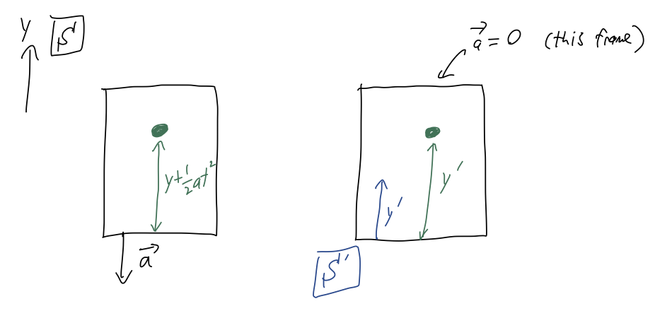
We drop a ball inside an elevator, from initial height \( y_0 \). From the point of view of frame \( \mathcal{S} \), fixed with respect to the ground, the elevator is moving straight down with constant acceleration \( a \). As pictured, we can define a second frame of reference \( \mathcal{S}' \) which is fixed to the elevator (so the point of view of an experimenter riding the elevator, basically.)
Let's work out the motion in frame \( \mathcal{S} \) first. Neglecting air resistance, the only force acting on the ball is gravity:
\[ \begin{aligned} \vec{F}_g = -mg\hat{y} \end{aligned} \]
Using Newton's second law,
\[ \begin{aligned} \vec{F}_{\rm net} = -mg \hat{y} = m\vec{a} = m(\ddot{x} \hat{x} + \ddot{y} \hat{y}) \end{aligned} \]
so nothing happens in the \( \hat{x} \)-direction, but vertically we have a constant acceleration, \( \ddot{y} = -g \). If we drop the ball at rest, integrating twice gives us
\[ \begin{aligned} y(t) = y_0 - \frac{1}{2} gt^2. \end{aligned} \]
So far, we haven't mentioned the elevator at all; it enters in when we ask how far the ball is from the floor of the elevator at any given time. From the diagram, we can see right away that
\[ \begin{aligned} \Delta y(t) = y(t) + \frac{1}{2} at^2 = y_0 + \frac{1}{2} (a-g) t^2. \end{aligned} \]
In particular, notice that if the elevator is also free falling (\( a=g \)), then the ball will appear to be suspended above the floor.
What about the frame \( \mathcal{S}' \)? Well, the only force in the problem is still gravity, so we conclude right away that
\[ \begin{aligned} y'(t) = y'_0 - \frac{1}{2} gt^2. \end{aligned} \]
\( y'(t) \) is exactly the same thing as \( \Delta y(t) \), the distance from the floor to the ball. But we don't see \( a \) anywhere, and in particular we don't see any possibility for the ball to be suspended in mid-air. This is a contradiction!
Obviously, one of our answers is wrong, and if you remember the fine print on Newton's laws, you may already know the answer: the calculation in \( \mathcal{S}' \) is wrong, because \( \mathcal{S}' \) is an accelerating frame of reference. Accelerating frames are also called non-inertial frames, because the law of inertia (Newton's first law) doesn't hold, and clearly neither does the second law.
The good news is that we're never forced to use a non-inertial frame, because frames of reference are our choice! Our calculation in the frame of an observer outside the elevator is perfectly fine. But it's an important point to be aware of. Unless we specify otherwise, for the rest of the semester we'll work only in inertial frames (i.e. non-accelerated ones where Newton's laws are good.)
There is, in fact, a way to modify Newton's laws so that they will work in an accelerating frame - this involves adding so-called 'fictitious force' terms. (If you've ridden in a fast elevator, you know these forces are something you can easily feel!) But that's a topic for next semester.
Newton's laws in curvilinear coordinates
Now that we've reviewed both Newton's laws and curvilinear coordinate systems, let's have a closer look at what happens when we put the two together. We'll focus mainly on cylindrical coordinates, which will show the important features; spherical is more complicated but not really different.
Remember that one of the nice things about Newton's laws in Cartesian coordinates is that they split apart into three separate equations for the \( x,y,z \) directions. Let's remind ourselves why: Newton's second law reads
\[ \begin{aligned} \vec{F} = m\ddot{\vec{r}} \\ F_x \hat{x} + F_y \hat{y} + F_z \hat{z} = m \frac{d^2}{dt^2} \left( x \hat{x} + y \hat{y} + z\hat{z} \right) \end{aligned} \]
and then acting with the time derivatives and matching components, we read off the individual equations \( F_x = m\ddot{x} \) and so on.
Now, we can do the same thing in cylindrical coordinates, using our results from above:
\[ \begin{aligned} F_\rho \hat{\rho} + F_\phi \hat{\phi} + F_z \hat{z} = m \frac{d^2}{dt^2} \left( \rho \hat{\rho} + z \hat{z} \right) \end{aligned} \]
You might be tempted to just starting matching terms again and conclude that \( F_\rho \stackrel{?}{=} m\ddot{\rho} \). But there's an immediate problem, which is that there doesn't seem to be a \( \hat{\phi} \) term on the right-hand side! Does this mean that \( F_\phi \) is just irrelevant, no matter how large the force is? (That seems like a strange conclusion...)
The resolution to this problem is that the simple argument above is ignoring some of the time dependence. We can see this by drawing two different vectors \( \vec{r}_1 \) and \( \vec{r}_2 \), and noting the directions of the unit vectors:
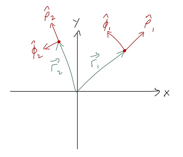
As we noted before, the direction of the cylindrical unit vectors is different for \( \vec{r}_1 \) and \( \vec{r}_2 \). But in the context of mechanics, \( \vec{r}_2 \) could represent a time-evolved version of \( \vec{r}_1 \) for some system, i.e. \( \vec{r}_1 = \vec{r}(t_1) \) and \( \vec{r}_2 = \vec{r}(t_2) \). If so, then it's obvious that the unit vectors \( \hat{\rho} \) and \( \hat{\phi} \) themselves must be time-dependent.
If you look at Taylor, he'll show you a nice geometric way to find the time derivatives. Instead of repeating him, I'll do it with algebra instead. Remember that we previously found these expressions for the cylindrical unit vectors:
\[ \begin{aligned} \hat{\rho} = \frac{d\vec{r}/d\rho}{|d\vec{r}/d\rho|} = \cos \phi \hat{x} + \sin \phi \hat{y} \\ \hat{\phi} = \frac{d\vec{r}/d\phi}{|d\vec{r}/d\phi|} = -\sin \phi \hat{x} + \cos \phi \hat{y} \end{aligned} \]
Now we can just take time derivatives explicitly, using the fact that \( \hat{x} \) and \( \hat{y} \) are time-independent. Starting with the radial direction,
\[ \begin{aligned} \frac{d\hat{\rho}}{dt} = -\dot{\phi} \sin \phi \hat{x} + \dot{\phi} \cos \phi \hat{y} \\ = \dot{\phi} \hat{\phi}, \end{aligned} \]
recognizing the form of the other unit vector and substituting it back in. Similarly, it's easy to show that
\[ \begin{aligned} \frac{d\hat{\phi}}{dt} = -\dot{\phi} \hat{\rho}. \end{aligned} \]
Now let's go back to Newton's second law and expand out the right-hand side. I'll ignore the \( z\hat{z} \) piece because it's the same as in Cartesian coordinates. What we need is, going slowly:
\[ \begin{aligned} \frac{d^2}{dt^2} \left( \rho \hat{\rho} \right) = \frac{d}{dt} \left( \dot{\rho} \hat{\rho} + \rho \frac{d\hat{\rho}}{dt} \right) \\ = \frac{d}{dt} \left( \dot{\rho} \hat{\rho} + \rho \dot{\phi} \hat{\phi} \right) \\ = \ddot{\rho} \hat{\rho} + \dot{\rho} \frac{d\hat{\rho}}{dt} + (\dot{\rho} \dot{\phi} + \rho \ddot{\phi}) \hat{\phi} + \rho \dot{\phi} \frac{d\hat{\phi}}{dt} \\ = \ddot{\rho} \hat{\rho} + \dot{\rho} \dot{\phi} \hat{\phi} + (\dot{\rho} \dot{\phi} + \rho \ddot{\phi}) \hat{\phi} - \rho \dot{\phi}^2 \hat{\rho} \\ = (\ddot{\rho} - \rho \dot{\phi}^2) \hat{\rho} + (\rho \ddot{\phi} + 2 \dot{\rho} \dot{\phi}) \hat{\phi} \end{aligned} \]
gathering together terms at the end. Putting this back into Newton's second law, we find the equations for the other two components:
\[ \begin{aligned} F_\rho = m(\ddot{\rho} - \rho \dot{\phi}^2) \\ F_\phi = m(\rho \ddot{\phi} + 2\dot{\rho} \dot{\phi}) \end{aligned} \]
The good news is that we now have dependence on all three coordinates, and on all three components of the force. The bad news is that this is going to give much more complicated differential equations for us to solve! (Attacking them directly, using the alternative Lagrangian formulation, is something you'll come back to next semester.)
Clicker Question(s)
Consider an object undergoing simple circular motion. Which of the four force components above is the "centripetal force", written as \( mv^2 / R \) in intro physics? Which of the four force components involves the "angular acceleration", \( \alpha = a_{\rm tangent} / R \)?
A. \( m \ddot{\rho} \)
B. \( m \rho \dot{\phi}^2 \)
C. \( m \rho \ddot{\phi} \)
D. \( 2m \dot{\rho} \dot{\phi} \)
E. A combination of more than one of the above
Answers: B is centripetal force, and C is angular acceleration.
First of all, the centripetal force \( mv^2 / R \) is in the radial direction, so it has to be either A or B. There are a few ways to see it has to be B; one is to remember that in intro physics, \( \rho = R \) is held fixed, so \( \ddot{\rho} \) is just zero. We can see it directly by noticing that the angular speed \( \omega = v/R \) is exactly \( \dot{\phi} \), so \( \rho \dot{\phi}^2 = R (v/R)^2 = v^2/R \), which is exactly the centripetal acceleration. (We can also see it from the minus sign: centripetal force should point towards the origin, so A has the wrong sign.)
For angular acceleration, \( \alpha \) is the rate of change of \( \omega \), in the same way that \( \omega \) is the rate of change of \( \phi \). Since \( a{\rm tangent} \) is in the \( \hat{\phi} \) direction, it is an acceleration that increases \( \phi \) only. (The division by \( R \) helps the units to make sense.) So \( \alpha = \ddot{\phi} \), which means term C is the one that involves angular acceleration.
There are specific problems where cylindrical coordinates are the best choice even for solving with Newton's laws. A good example is a simple pendulum:
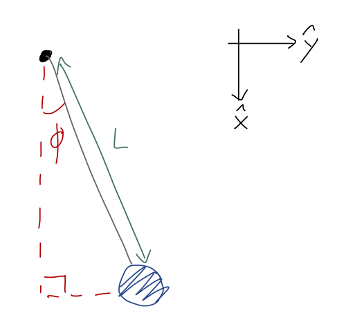
Note that I've turned the coordinates around a bit compared to how we usually draw them; this is so that I can identify the angle \( \phi = 0 \) with the lowest point of the pendulum. (Again, physical intution: we know that hanging straight down is a special point because the pendulum won't move if we start it there. So we anticipate the answer will be a bit simpler with these coordinates.)
For the pendulum, the cylindrical radius is fixed to the length of the string, \( \rho = L \). This means that any time derivatives of \( \rho \) vanish, leaving us with the equations
\[ \begin{aligned} F_\rho = -mL \dot{\phi}^2 \\ F_\phi = mL \ddot{\phi} \end{aligned} \]
Notice, by the way, that if we were studying purely circular motion (e.g. the pendulum is being spun around on a flat surface instead of hanging vertically), we would have \( \dot{\phi} = v/L \), and the first equation becomes
\[ \begin{aligned} F_\rho = -mL \left( \frac{v}{L} \right)^2 = -m\frac{v^2}{L} \end{aligned} \]
which is the familiar equation for centripetal force. (By assumption of circular motion, the angular speed \( \dot{\phi} \) is constant, so the second equation is just \( F_\phi = 0 \).)
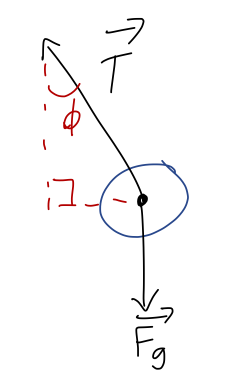
Back to the more general case of a pendulum. We should draw a free-body diagram:
Let's get some practice working in cylindrical coordinates.
Clicker Question
(note: we skipped this one in class.)
What is \( T_\phi \), the component of tension in the \( \hat{\phi} \) direction?
A. \( T \)
B. \( T \cos \phi \)
C. \( T \sin \phi \)
D. \( 0 \)
Answer: D
Let's draw angles onto our free-body diagram and identify the unit-vector directions:
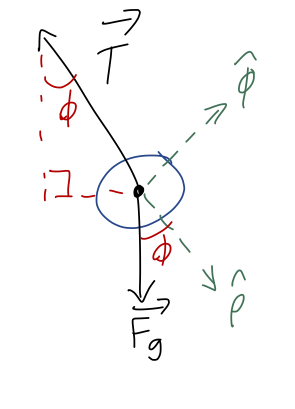
We immediately see that \( \hat{\phi} \) is perpendicular to \( T \), which means that \( T_\phi \) is zero! This is one of the nice things about using cylindrical coordinates for this problem, the fact that the vector expression for tension is always the same,
\[ \begin{aligned} \vec{T} = -T \hat{\rho}, \end{aligned} \]
regardless of where the pendulum is.
As for gravity, we will need to decompose it into radial and tangential pieces. This time I'll do it the geometric way, but note that you can also start with \( F_g = -mg\hat{y} \) and use algebra as an alternative way to convert. (Try it out if you're not comfortable with vector algebra yet!) From the sketch above, we readily find that
\[ \begin{aligned} \vec{F}_g = mg \cos \phi \hat{\rho} - mg \sin \phi \hat{\phi} \end{aligned} \]
Now we can plug back in to Newton's laws in cylindrical components. Combining the radial forces, the first equation reads
\[ \begin{aligned} mg \cos \phi - T = -mL \dot{\phi}^2 \end{aligned} \]
and the second is
\[ \begin{aligned} -mg \sin \phi = mL \ddot{\phi}. \end{aligned} \]
To solve for the motion, we can completely ignore the first equation, because it contains the unknown tension force \( T \). (If we care about the tension, like if we know our string has a max tension and we want to predict whether it will break, we can go back and check at the end once we know \( \phi(t) \).) The second equation simplifies slightly to:
\[ \begin{aligned} \ddot{\phi} = -\frac{g}{L} \sin \phi. \end{aligned} \]
Let's check units, always a good practice: \( \phi \) is dimensionless, \( g \) has units of \( m/s^2 \), and \( L \) has units of \( m \), so we have \( 1/s^2 \) on the right. This matches the left exactly, because \( d/dt \) itself has units of \( 1/s \). (If this isn't clear to you, think about the basic definition of a derivative: \( du/dt \) comes from the infinitesmal limit of \( \Delta u / \Delta t \), and the units of \( \Delta t \) are clearly the same as the units of \( t \).)
In this case both sides depend on the unknown \( \phi \), so we can't just integrate with respect to time. In fact, this is actually a surprisingly hard differential equation to solve, for such a simple system! There is no analytic solution in terms of elementary functions in general, but we can find an approximate solution: if we assume the angle \( \phi \) is always small (the 'small-angle approximation'), then we can Taylor expand the right-hand side about \( \phi=0 \),
\[ \begin{aligned} \sin \phi \approx \phi\ + ... \end{aligned} \]
giving the simpler equation
\[ \begin{aligned} \ddot{\phi} = -\frac{g}{L} \phi. \end{aligned} \]
This still depends on \( \phi \) on both sides, but it has a relatively simple general solution, of the form
\[ \begin{aligned} \phi(t) = A \sin (\omega t) + B \cos (\omega t) \end{aligned} \]
where \( \omega = \sqrt{g/L} \). At this point, we're not ready to study how to get that general solution yet, but it's easy for you to plug it back in and check that it works.
We're starting to see that there are examples of equations of motion where the forces depend on coordinates, and we can't just solve by simply integrating. In fact, this is a great point for us to go back to math, and start to study the more general theory of differential equations.