Ordinary differential equations
As we've started to see, solving equations of motion in general requires the ability to deal with more general classes of differential equations than the simple examples from first-year physics. Before we go back to mechanics, let's start to think about the general theory of differential equations and how to solve them.
Specifically, we'll begin with the theory of ordinary differential equations, or "ODEs". The opposite of ordinary is a partial differential equation, or "PDE", which contains partial derivatives; an ordinary DE has only regular (total) derivatives, or in other words, all of the derivatives are with respect to one and only one variable. Newtonian mechanics problems are always ODEs, because we only have derivatives with respect to time in the second law.
Now, a very important fact about differential equations is that their solutions alone are not unique; we need more information to find a complete solution. As a simple example, consider the equation
\[ \begin{aligned} \frac{dy}{dx} = 2x \end{aligned} \]
You can probably guess right away that the function \( y(x) = x^2 \) satisfies this equation. But so does \( y(x) = x^2 + 1 \), and \( y(x) = x^2 - 4 \), and so on! In fact, this equation is simple enough that we can integrate both sides to solve it:
\[ \begin{aligned} \int dx \frac{dy}{dx} = \int dx 2x \\ y(x) = x^2 + C \end{aligned} \]
remembering to include the arbitrary constant of integration for these indefinite integrals. So the equation alone is not enough to give us a unique solution. But in order to fix the constant \( C \), we just need a single extra piece of information. For example, if we add the condition
\[ \begin{aligned} y(0) = 1 \end{aligned} \]
then \( y(x) = x^2 + 1 \) is the only function that will work.
What if we have a second-order derivative to deal with, like in Newton's second law \( \vec{F} = m \ddot{\vec{r}} \)? To solve this equation (or indeed any ODE that has a second-order derivative), we will need two conditions to find a unique solution. One way to think of this is to think about solving the equation by integration; to reverse both derivatives on \( d^2 \vec{r} / dt^2 \), we have to integrate twice, getting two constants of integration to deal with.
This statement turns out to be true in general, even though we can't solve most ODEs just by integrating directly: every derivative that has to be reversed gives us one new unknown constant of integration. Notice that I've been using a calculus vocabulary term, which is 'order': the object
\[ \begin{aligned} \frac{d^{(n)} f}{dx^n} = \left( \frac{d}{dx} \right)^n f(x) \end{aligned} \]
is called the \( n \)-th order derivative of \( f \) with respect to \( x \). The same vocabulary term applies to ODEs: the order of an ODE is equal to the highest derivative order that appears in it. (So Newton's second law is a second-order ODE; to solve it we need two conditions, usually the initial position and initial velocity.)
Here's another way to understand how order relates to the number of conditions. Using Newton's law as an example again, notice that in full generality, we can rewrite it in the form
\[ \begin{aligned} \frac{d^2 \vec{r}}{dt^2} = f\left(\vec{r}, \frac{d \vec{r}}{dt} \right). \end{aligned} \]
In other words, if at any time \( t \) we know both the position and the velocity, then we can just plug in to this equation to find the acceleration at that time. But then because acceleration is the time derivative of velocity, we can predict what will happen next! Suppose we start at \( t=0 \). Then a very short time later at \( t = \epsilon \),
\[ \begin{aligned} \frac{d\vec{r}}{dt}(\epsilon) = \frac{d\vec{r}}{dt}(0) + \epsilon \frac{d^2 \vec{r}}{dt^2}(0) + ... \\ \vec{r}(\epsilon) = \vec{r}(0) + \epsilon \frac{d\vec{r}}{dt}(0) + ... \end{aligned} \]
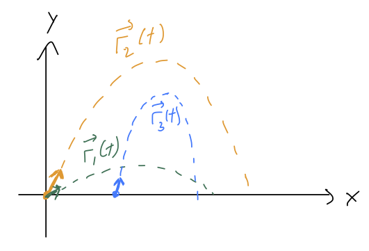
Now we know the 'next' values of position and velocity for our system. And since we know those, we plug in to the equation above and get the 'next' acceleration, \( d^2 \vec{r} / dt^2(\epsilon) \). Then we repeat the process to move to \( t = 2\epsilon \), and then \( 3\epsilon \), and so on until we've evolved as far as we want to in time. Depending on what choices we made for the initial values, we'll build up different curves for \( \vec{r}(t) \):
This might sound like a tedious procedure, and it is, but this process (or more sophisticated versions of it) are exactly how numerical solution of differential equations are found. If you use the "NDSolve" function in Mathematica, for instance, it's doing some version of this iterative procedure to give you the answer. But more importantly, I think this is a more physical way to think about what initial conditions mean, and why we need \( n \) of them for an \( n \)-th order ODE.
As a side benefit, this construction also established uniqueness of solutions, meaning that once we fully choose the initial conditions, there is only one possible answer for the solution to the ODE. For Newtonian physics, this means that knowing the initial position and velocity is enough to tell you the unique possible physical path \( \vec{r}(t) \) that the system will follow.
Keep in mind that the construction above makes use of initial values, where we specify all of the conditions on our ODE at the same point (same value of \( t \) here.) This is a special case of the more general idea of boundary conditions, which can be specified in different ways. (For example, we could find a unique solution for projectile motion by specifying \( y(0) = y(t_f) = 0 \) and solving from there to see when our projectile hits the ground again.)
Classifying ODEs and general solutions
Numerical solution is a great tool, but whenever possible we would prefer to be able to solve the equation by hand - this is more powerful because we can solve for a bunch of initial conditions at once, and we can have a better understanding of what the solution means.
This brings us to classification of differential equations. There is no algorithm for solving an arbitrary differential equation, even an ODE, and many such equations have no known solutions at all (at which point we go back to numerics.) But there is a long list of special cases in which a solution is known, or a certain simplifying trick will let us find one. Because analytic solution of ODEs is all about knowing the special cases, it's very important to recognize whether a given equation we find in the wild belongs to one of the classes we have some trick for.
The first such classification we'll go learn to recognize is the linear ODE (the opposite of which is nonlinear.) To explain this clearly, remember that a linear function is one of the form
\[ \begin{aligned} y(x) = mx + b. \end{aligned} \]
To state this in words, the function only modifies \( x \) by addition and multiplication with some constants, \( m \) and \( b \). A linear differential equation, then, is one in which the unknown function and its derivatives are only multiplied by constants and added together.
For example, if we're solving for \( y(x) \), the most general linear differential equation looks like
\[ \begin{aligned} a_0(x) y + a_1(x) \frac{dy}{dx} + a_2(x) \frac{d^2y}{dx^2} + ... + b(x) = 0. \end{aligned} \]
This is a little more complicated since we have two variables now, but if you think of freezing the value of \( x \), then all of the \( a \)'s and \( b \) are constant and it's clearly a linear function.
Clicker Question
Which of the following ODEs are linear?
\( \frac{dy}{dx} + 3y = 1 \)
\[\frac{d^2u}{dt^2} + \sin^2 (t) u = 0\]
\( \frac{dy}{dx} + \frac{3}{y} = 1 \)
A. Only 1 is linear.
B. 1 and 2 are linear.
C. 1 and 3 are linear.
D. All of them are linear.
E. None of them are linear.
Answer: B
This is just a check to help you understand the definition of a linear ODE. Recall that in a linear ODE, the unknown function (the one we're taking derivatives of) can only appear linearly, i.e. multiplied by constants or added together.
Based on this definition, 1) is definitely linear: the unknown \( y \) either appears alone (in \( dy/dx \)) or multiplied by terms which are obviously constant. 2) is a little trickier, but it is also linear: although \( \sin^2(t) \) doesn't look like a "constant", the key is that it doesn't depend on \( u \) at all.
On the other hand, although it looks relatively simple, 3) is not linear. This is because of the \( 3/y \) term, which doesn't amount to just multipyling \( y \) by constants. (You might think of trying to multiply through by \( y \) to simplify this, but it won't help here, because we would end up with the term \( y \cdot dy/dx \) which is still not linear.)
Linearity turns out to be a very useful condition. This isn't a math class so I won't go over the proof, but there is a very important result for linear ODEs:
_A linear ODE of order \( n \) has a unique general solution which depends on \( n \) independent unknown constants._
The term "general solution" means that there is a function we can write down which solves the ODE, no matter what the initial conditions are. This function has to contain \( n \) constants that can be adjusted to match initial conditions (as we discussed above), but otherwise it is the same function everywhere.
(To avoid a common misconception, it's just as important to be aware of the opposite of this statement: if we have non-linear ODE, in many cases there is no general solution. There is still always a unique solution if we fully specify the initial values. But for a non-linear ODE the functional form of the solution can be different depending on what the initial values are! See Boas 8.2 for an example.)
Alright, so it's great that we know a general solution is out there, but how do we find it in practice? It's probably best to explain this using an example.
Example: a simple linear ODE
Let's solve the following ODE:
\[ \begin{aligned} \frac{d^2y}{dx^2} = +k^2 y \end{aligned} \]
There is a general procedure for solving second-order linear ODEs like this, but I'll defer that until later. To show off the power of general solutions, I'm going to use a much cruder approach: guessing. (If you want to sound more intellectual when you're guessing, the term used by physicists for an educated guess is "ansatz".)
Notice that the equation tells us that when we take the derivative of \( y(x) \) twice, we end up with a constant times \( y(x) \) again. This should immediately make you think about exponential functions, since \( d(e^x)/dx = e^x \). To get the constant \( k \) out from the derivatives, it should appear inside the exponential. So we can guess
\[ \begin{aligned} y_1(x) = e^{+kx} \end{aligned} \]
and easily verify that this indeed satisfies the differential equation. However, we don't have any arbitrary constants yet, so we can't properly match on to initial conditions. We can notice next that because \( y(x) \) appears on both sides of the ODE, we can multiply our guess by a constant and it will still work. So our refined guess is
\[ \begin{aligned} y_1(x) = Ae^{+kx}. \end{aligned} \]
This is progress, but we have only one unknown constant and we need two. Going back to the equation, we can notice that because the derivative occurs twice, a negative value of \( k \) would also satisfy the equation. So we can come up with a second guess:
\[ \begin{aligned} y_2(x) = Be^{-kx}. \end{aligned} \]
This is very similar to our first guess above, but it is in fact an independent solution, independent meaning that we can't just change the values of our arbitrary constants to get this form from the other solution. (We're not allowed to change \( k \), because it's not arbitrary, it's in the ODE that we're solving!)
Finally, we notice that the combination \( y_1(x) + y_2(x) \) of these two solutions is also a solution if we plug it back in. So we have
\[ \begin{aligned} y(x) = Ae^{+kx} + Be^{-kx} \end{aligned} \]
This is a general solution: it's a solution and it has two distinct unknown constants, \( A \) and \( B \). Thanks to the math result above, if we have a general solution to a linear ODE, we know that it is the general solution thanks to uniqueness.
The whole procedure we just followed might seem sort of arbitrary, and indeed it was, since it was based on guessing! For different classes of ODEs, there will be a variety of different solution methods that we can use. The power of the general solution for linear ODEs is that no matter how we get there, once we find a solution with the required number of arbitrary constants, we know that we're done. Often it's easiest to find individual functions that solve the equation, and then put them together as we did here. (Remember, solving ODEs is all about recognizing special cases and equations you've seen before!)
Clicker Question
Suppose that we have the initial condition \( y(0) = 0 \) for the ODE we just solved. What does this tell us about the behavior of \( y(x) \) at very large, positive \( x \)?
\[ \begin{aligned} y(x) = Ae^{+kx} + Be^{-kx} \end{aligned} \]
A. \( y(x) \) blows up (increases without bound to \( \pm \infty \).)
B. \( y(x) \) vanishes (decreases towards zero.)
C. \( y(x) \) is always zero.
D. \( y(x) \) approaches a constant value (but we need another condition to find that value.)
E. Either A or C could be true, depending on the other condition.
Answer: E
Although it is true that we need two initial conditions to find both \( A \) and \( B \), the only way to decide what the one condition we're given tells us is to plug it in (it will give us some relationship between \( A \) and \( B \), allowing us to eliminate one of them.) Let's try it:
\[ \begin{aligned} y(0) = 0 = A + B \end{aligned} \]
so we find the simple condition that \( A = -B \). We can then plug back in to the equation to eliminate \( B \), finding
\[ \begin{aligned} y(x) = A (e^{+kx} - e^{-kx}). \end{aligned} \]
At very large, positive \( x \), the \( e^{-kx} \) term goes to zero, so we can ignore it compared to the \( e^{+kx} \) which will become very large. Thus, we find that \( y(x) \) will blow up as \( x \) becomes very large - unless \( A = 0 \)! If the other initial condition gives us \( A=0 \), then we just have \( y(x) = 0 \), which is answer C instead. So E is correct.
(The case where \( y(x) = 0 \) everywhere is not very interesting - mathematicians would call this the "trivial solution". But we need one more initial condition to decide either way!)