Now let's start to look at some specific methods for solving differential equations. We're going to begin with first-order ODEs only, because that will open up a new class of physics problems for us to solve: projectile motion with air resistance. Later in the semester, we'll come back to second-order ODEs.

Linear first-order ODEs

(Note: this solution is discussed in Boas 8.3, but I'm borrowing a little bit of terminology from later sections of chapter 8 to put it in context.)

It turns out that there is a nice and general way to find solutions linear first-order ODEs. The combination of linear and first-order is very restrictive: any such ODE must take the form

\[ \begin{aligned} \frac{dy}{dx} + P(x) y = Q(x). \end{aligned} \]

This is a good place to introduce one last technical term, which is homogeneous. A homogeneous ODE is one in which every single term depends on the unknown function \( y \) or its derivatives. The equation above does not satisfy this condition, because the \( Q(x) \) term on the right doesn't have any \( y \)-dependence; thus, we say this equation is inhomogeneous (some books will use "nonhomogeneous" instead.)

Now, there is another equation which closely related to the one above:

\[ \begin{aligned} \frac{dy_c}{dx} + P(x) y_c = 0. \end{aligned} \]

The "c" here stands for complementary; this equation is called the complementary equation to the original. Setting \( Q(x) \) to zero gives us an equation that is homogeneous. Better yet, this equation is separable too: we can readily find that

\[ \begin{aligned} \frac{dy_c}{y_c} = -P(x) dx \end{aligned} \]

or doing the integrals,

\[ \begin{aligned} y_c(x) = A e^{-\int dx P(x)}. \end{aligned} \]

Of course, this is only a solution if \( Q(x) \) happens to be zero. But it turns out to be part of the solution for any \( Q(x) \). Suppose that we are able to find some other function \( y_p(x) \), which is a particular solution that satisfies the original, inhomogenous equation. Then \( y(x) = y_c(x) + y_p(x) \) is also a solution of the full equation. This is easy to see by plugging in:

\[ \begin{aligned} \frac{dy}{dx} + P(x) y = \frac{d}{dx} \left( y_c(x) + y_p(x) \right) + P(x) (y_c(x) + y_p(x)) \\ = \left[\frac{dy_c}{dx} + P(x) y_c(x) \right] + \left[ \frac{dy_p}{dx} + P(x) y_p(x) \right] \\ = 0 + Q(x). \end{aligned} \]

This might not seem very useful, because we still have to find \( y_p(x) \) somehow. But notice that \( y_c(x) \) always has the arbitrary constant \( A \) in it. That means that \( y(x) = y_c(x) + y_p(x) \) is the general solution to our original ODE (the unique one, because it's linear, remember!)

Example: charging a capacitor

This isn't a mechanics example, but it happens to be one of the simpler cases of a first-order and inhomogeneous ODE problem, so let's do it anyway. We have an electric circuit consisting of a battery supplying voltage \( V_0 \), a resistor with resistance \( R \), and a capacitor with capacitance \( C \):

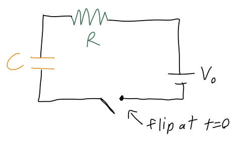
If the capacitor begins with no charge at \( t=0 \), we want to describe the current \( I(t) \) flowing in the circuit as a function of time. Now, current is the flow of charge, so the charge \( Q \) on the capacitor will satisfy the equation

\[ \begin{aligned} I = \frac{dQ}{dt}. \end{aligned} \]

The other relevant circuit equations we need are \( V = IR \) for the resistor, and \( Q = CV \) for the capacitor. Putting these together, we find that the equation describing the circuit is

\[ \begin{aligned} R \frac{dQ}{dt} + \frac{Q}{C} = V_0. \end{aligned} \]

The complementary equation is

\[ \begin{aligned} R\frac{dQ_c}{dt} + \frac{Q_c}{C} = 0 \end{aligned} \]

which is nice and separable:

\[ \begin{aligned} \frac{dQ_c}{Q_c} = -\frac{1}{RC} dt \end{aligned} \]

Integrating gives

\[ \begin{aligned} \ln Q_c = -\frac{t}{RC} + K \Rightarrow Q_c(t) = K' e^{-t/(RC)} \end{aligned} \]

Now we need to find the particular solution \( Q_p \). Fortunately, because the right-hand side is just a constant, it's easy to see that a constant value for \( Q_p \) will give us what we want. Specifically, if

\[ \begin{aligned} Q_p = CV_0 \end{aligned} \]

then the equation is satisfied, since the derivative term just vanishes.

Finally, we put things together and apply our boundary condition, \( Q(0) = 0 \):

\[ \begin{aligned} Q_c(0) + Q_p(0) = 0 = K' e^{-0/(RC)} + CV_0 = K' + CV_0 \end{aligned} \]

finding that \( K' = -CV_0 \), and thus the finished result is

\[ \begin{aligned} Q(t) = CV_0 \left(1 - e^{-t/(RC)} \right). \end{aligned} \]

So far, everything I've said is actually fairly general: this same approach with complementary and particular solutions will be something we use a lot when we get to second-order ODEs.

For any first-order linear ODE, there is actually a trick which will always give you the particular solution for any functions \( P(x) \) and \( Q(x) \). However, it's a little complicated to write down, and we won't need it often. So I won't cover that here, and instead I'll refer you to Boas 8.3 for the result. This is one of those formulas that you should know exists, but it's not worth memorizing - if you find you need it, you can go look it up.

Separable first-order ODEs

A unique feature of first-order ODEs is that we can sometimes solve them just by doing integrals. A first-order ODE is separable if we can write it in the form

\[ \begin{aligned} F(y) dy = G(x) dx \end{aligned} \]

where \( F(y) \) and \( G(x) \) are just any arbitrary function. Once we've reached this form, we can just integrate both sides and end up with an equation relating \( y \) to \( x \), which is our solution.

A quick aside: splitting the differentials \( dy \) and \( dx \) apart like this is something physicists tend to do much more than mathematicians (although Boas does it!) Remember that \( dx \) and \( dy \) do have meaning on their own, as they're defined to be infinitesmal intervals when we define the derivative \( dy/dx \). That being said, if you're unsettled by the split derivative above, you can instead think of a separable ODE as one written in the form

\[ \begin{aligned} F(y) \frac{dy}{dx} = G(x) \end{aligned} \]

Then we can integrate both sides over \( dx \),

\[ \begin{aligned} \int F(y) \frac{dy}{dx} dx = \int G(x) dx \end{aligned} \]

The integral on the left becomes \( \int F(y) dy \) by a \( u \)-substitution. After we do the integrals, we just have a regular equation to solve for \( y \). The simplest case is when \( F(y) = 1 \), i.e. if we have

\[ \begin{aligned} \frac{dy}{dx} = G(x) \\ \int dy = \int G(x) dx \\ y = \int G(x) dx + C \end{aligned} \]

(notice that we get one overall constant of integration from the indefinite integrals, just as needed to match the single initial condition for a first-order ODE.)

Let's try a more interesting example.

Example: a separable first-order ODE

We'll solve the following ODE:

\[ \begin{aligned} x \frac{dy}{dx} - y = xy \end{aligned} \]

This might not be obviously separable, but let's do some algebra to find out. We'll put the \( y \)'s together first:

\[ \begin{aligned} x \frac{dy}{dx} = y(1+x) \end{aligned} \]

Then divide by \( x \) and by \( y \):

\[ \begin{aligned} \frac{1}{y} \frac{dy}{dx} = \frac{1+x}{x} \end{aligned} \]

Nice and separated! Next, we split the derivative apart and integrate on both sides:

\[ \begin{aligned} \int \frac{dy}{y} = \int dx\ \frac{1+x}{x} \end{aligned} \]

The left-hand side integral will give us the log of \( y \). On the right, it's easiest to just divide out and write it as \( 1/x + 1 \), which gives us two simple integrals:

\[ \begin{aligned} \ln y + C' = \int dx\ \left(1 + \frac{1}{x} \right) = x + \ln x + C'' \end{aligned} \]

Just to be explicit, I kept both unknown constants here since we did two indefinite integrals. But since \( C' \) and \( C'' \) are both arbitrary, and we're adding them together, we can just combine them into a single constant \( C = C'' - C' \).

Now we need to solve for \( y \). Start by exponentiating both sides:

\[ \begin{aligned} y(x) = \exp \left( x + \ln x + C'' \right) \\ = e^x e^{\ln x} e^{C''} \\ = B x e^x \end{aligned} \]

defining one more arbitrary constant. (Since we haven't determined what the constant is yet by applying boundary conditions, it's not so important to keep track of how we're redefining it.)

Finally, we can impose a boundary condition to find a particular solution. Let's say that \( y(2) = 2 \). We plug in to get an equation for \( B \):

\[ \begin{aligned} y(2) = 2 = 2B e^2 \\ \Rightarrow B = \frac{1}{e^2} = e^{-2} \end{aligned} \]

and so

\[ \begin{aligned} y(x) = xe^{x-2}. \end{aligned} \]

Clicker Question

How should we solve the following equation?

\[ \begin{aligned} m \frac{dv}{dt} = -cv^2 \end{aligned} \]

A. It's first-order and homogeneous, a simple exponential solution will work.

B. It's first-order and linear, we need to find complementary and particular solutions.

C. It's first-order and separable, we need to separate and integrate both sides.

D. It's second-order, we'll need some new method to solve it.

Answer: C

For those of you who have finished the reading already, you'll recognize this as the equation for quadratic air resistance. It is indeed first-order; don't let the \( v^2 \) fool you, only the number of derivatives matters for order! It's also non-linear, which is bad news for many of our solution techniques. But the good news is that it is separable, and separability doesn't care about linearity.

In fact, since there is no explicit \( t \)-dependence at all, it's easy to separate out:

\[ \begin{aligned} \frac{dv}{v^2} = -\frac{c}{m} dt \end{aligned} \]

Now we integrate:

\[ \begin{aligned} -\frac{1}{v} = -\frac{c}{m} t + C' \end{aligned} \]

and invert:

\[ \begin{aligned} v(t) = \frac{1}{(c/m) t - C'} \end{aligned} \]

Now we have to apply a boundary condition to fix \( C' \). (We could also have done this before solving for \( v(t) \), the order doesn't matter.) Let's take the initial condition \( v(0) = v_0 \). Plugging in at \( t=0 \) gives a nice and simple relation,

\[ \begin{aligned} v(0) = v_0 = \frac{1}{-C'} \end{aligned} \]

or \( C' = -1/v_0 \). This gets rid of our last minus sign, and we find for the result

\[ \begin{aligned} v(t) = \frac{1}{(c/m)t + 1/v_0} = \frac{v_0}{1 + \frac{cv_0}{m} t}. \end{aligned} \]

We'll talk about the implications of this solution more once we've set up the physics context for air resistance properly.

Projectile motion and air resistance

Let's come back to physics and put our theory of first-order ODEs to use. Air resistance problems turn out to be the perfect application, because air resistance gives a force which depends on the velocity of the object moving through the air. Of course, Newton's second law is generally a second-order ODE,

\[ \begin{aligned} \vec{F} = m\ddot{\vec{r}}. \end{aligned} \]

But in the special case that the force only depends on the velocity \( \vec{v} = d\vec{r}/dt \), we can rewrite this as

\[ \begin{aligned} \vec{F}(\vec{v}) = m\dot{\vec{v}} \end{aligned} \]

which we can treat as a first-order ODE.

Before we get to the math, let's talk about the physics of air resistance, also known as drag for short (not to be confused with the regular friction that you get if you drag an object across a rough surface.) As the name implies, this is a force which resists motion, which explains why it depends on speed.

What do we know about the nature of the drag force \( \vec{f}(\vec{v}) \)? First of all, the air is (to a very good approximation) isotropic, i.e. it is uniform enough that it looks the same no matter which direction we move through it.

This means that the magnitude of the drag force should only depend on the speed, i.e. \( \vec{f}(\vec{v}) = \vec{f}(v) \). If the object moving through the air is also very symmetrical (like a sphere), then the orientation of our object also doesn't matter, and we expect the direction of the force to be opposite the direction of motion,

\[ \begin{aligned} \vec{f}(v) = -f(v) \hat{v}. \end{aligned} \]

There are many examples of systems for which this second equation does not hold. Taylor gives the example of an airplane, which experiences a lift force clearly not in the same direction of its motion. A more mundane example is a frisbee, for which air resistance actually provides a stabilizing force that keeps it from tumbling while in the air. But there are lots of interesting systems where this relation does hold, so we'll assume it for the rest of this section.

Unfortunately, this is still way too general: we need some information about what the function \( f(v) \) is before we can hope to make any progress. There are two effects that are important in the interactions between a fluid and an object traveling through it, and they will give us linear and quadratic dependence on the speed respectively. So the most general drag force we will study is

\[ \begin{aligned} f(v) = bv + cv^2. \end{aligned} \]

Now, Taylor points out that this is valid at "lower speeds", and that there are other effects that are important near the speed of sound. In fact, another way to derive this form for \( f(v) \) is through Taylor series expansion. But we should be careful, because this is a physics class, and series expanding in \( v \) doesn't really make sense - it has units! If we really want to expand, we need to expand in something dimensionless; equivalently, we need to answer the question "\( v \) is small compared to what?"

The answer is what I already said: \( v \) should be small compared to \( v_s \), the speed of sound of air (or whatever fluid medium we are studying.) \( v_s \) is the speed at which the motion of the air molecules relative to each other will start to matter and things will get more complicated. Thus, we can write

\[ \begin{aligned} f(v) = b_0\frac{v}{v_s} + c_0 \frac{v^2}{v_s^2} + d_0 \frac{v^3}{v_s^3} + ... \end{aligned} \]

(there is no constant term \( a_0 \), for the simple reason that we know there is no drag force if \( v=0 \).) The beauty of this approach is that so long as we are working at speeds \( v \ll v_s \), we can study air resistance even if we have no idea what the original function \( f(v) \) is: all we have to do is run a few experiments to measure the constants \( b_0, c_0, d_0 \) (and so on, if we care about even smaller corrections.)

This is an example of the concept of an effective theory: the series expansion version of \( f(v) \) is not valid at any speed, but at small speeds it can be used to make useful predictions once we've done a couple experiments to set it up. This should all remind you of the classical limit \( v \ll c \) from special relativity, too. I'll come back to the idea of effective theories again later on, but I want to point it out here because it's more common than you think.