Let's continue our discussion of Taylor series starting with an example.
Example: a simple Taylor series
Let's do a simple example: we'll find the Taylor series expansion of
\[ \begin{aligned} f(x) = \sin^2(x) \end{aligned} \]
up to second order. We start by calculating derivatives:
\[ \begin{aligned} f'(x) = 2 \cos (x) \sin(x) \\ f''(x) = -2 \sin^2 (x) + 2 \cos^2(x) \end{aligned} \]
This gives us enough to find the Taylor series to quadratic order about any point we want. For example, we can do \( x = \pi/4 \), where \( \cos(\pi/4) = \sin(\pi/4) = 1/\sqrt{2} \). Then
\[ \begin{aligned} f'(\pi/4) = 1 \\ f''(\pi/4) = 0 \end{aligned} \]
and the general formula gives us
\[ \begin{aligned} \sin^2(x) \approx \frac{1}{2} + \left(x - \frac{\pi}{4} \right) + \mathcal{O}((x-\pi/4)^3) \end{aligned} \]
This introduces the big-O notation, which denotes order: it says that all of the missing terms are at least of order \( (x-\pi/4)^3 \), i.e. they're proportional to \( (x-\pi/4)^3 \) or even higher powers. I'm writing it explicitly here instead of just \( (...) \), because I want to make it clear that we know the quadratic term is zero.
If we expand at \( x=0 \) instead, then \( \sin(0) = 0 \) and \( \cos(0) = 1 \) gives
\[ \begin{aligned} f'(0) = 0 \\ f''(0) = 2 \end{aligned} \]
and thus
\[ \begin{aligned} \sin^2(x) \approx 0 + 0 x + \frac{1}{2!} (2) x^2 + ... = x^2 + \mathcal{O}(x^3). \end{aligned} \]
A couple more interesting things to point out here. First, we could have predicted that there would be no \( x \) term here: we know from the original function that \( \sin^2(-x) = \sin^2(x) \). But a linear term would be different at \( x \) and \( -x \), so its coefficient has to be zero. In fact, this extends to all odd powers: we know in advance there will be no \( x^3 \) term, no \( x^5 \) term, and so on.
Second, notice that we would have found the same answer if we started with the Taylor expansion of \( \sin(x) \) at zero,
\[ \begin{aligned} \sin(x) \approx x - \frac{x^3}{6} + ... \end{aligned} \]
and just squared it:
\[ \begin{aligned} \left(x - \frac{x^3}{6} + ... \right)^2 = x^2 - \frac{1}{3} x^4 + \frac{x^6}{36} + ... \\ \end{aligned} \]
and up to the first two terms, we find that the expansions match. (If we went back and found the \( x^6 \) terms above, we'd find that one matches too.)
This is not a coincidence, but a completely general result: one way to find Taylor series for functions of functions is just to start with a simple Taylor series, and then apply other functions to it. Remember, the Taylor series is a representation of the function: \( f(x)^2 \) and \( \left(\sum_n (...) \right)^2 \) really are the same thing! We just have to be careful with keeping track of terms up to the order in \( x \) to which we want to work.
(Boas is more enthusiastic about this trick, so you can look at her chapter 1.13 for more examples. Whether it's useful depends on the problem and on your own taste - personally I never liked polynomial long division, so I wouldn't use this for dividing two functions!)
Clicker Question
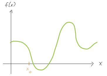
Consider a Taylor expansion of \( f(x) \) in the sketch above around point \( x_0 \),
\[ \begin{aligned} f(x) = a_0 + a_1 (x - x_0) + a_2 (x - x_0)^2 + ... \end{aligned} \]
Which statement is definitely true about the signs of \( a_0 \) and \( a_1 \)?
A. \( a_0 \) is positive, \( a_1 \) is positive
B. \( a_0 \) is positive, \( a_1 \) is negative
C. \( a_0 \) is negative, \( a_1 \) is positive
D. \( a_0 \) is negative, \( a_1 \) is negative
E. None of the above.
Answer: B
We can read this off the plot. First of all, \( a_0 \) is just the value of the function at point \( x_0 \), which we can clearly see is positive (above the axis.) So \( a_0 > 0 \). For the next term, \( a_1 \) is the slope of the line which most closely approximates \( f(x) \) near \( x = x_0 \). Since the function is sloping downwards here, we see that \( a_1 < 0 \) - the slope is negative.
Clicker Question
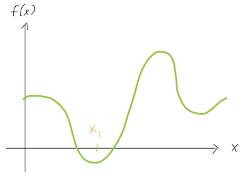
Consider a Taylor expansion of \( f(x) \) in the sketch above around point \( x_1 \),
\[ \begin{aligned} f(x) = a_0 + a_1 (x - x_1) + a_2 (x - x_1)^2 + ... \end{aligned} \]
Which statement is definitely true about the signs of \( a_1 \) and \( a_2 \)?
A. \( a_1 \) is positive, \( a_2 \) is positive
B. \( a_1 \) is positive, \( a_2 \) is negative
C. \( a_1 \) is negative, \( a_2 \) is positive
D. \( a_1 \) is negative, \( a_2 \) is negative
E. None of the above.
Answer: E
Same reasoning as above, except now we have \( a_2 \) instead of \( a_0 \). For \( a_2 \), we can imagine approximating \( f(x) \) close to \( x_1 \) by a parabola, so the sign will be determined by whether the parabola opens up (positive) or down (negative). Here the function opens upwards, so we must have \( a_2 \) positive. (You can also think in terms of derivatives: the slope, or first derivative, is changing from negative to positive here. So \( a_2 \), which is the second derivative and thus the rate of change of slope, must be positive.)
However, this is a local minimum of the function, so the slope of a line drawn through point \( x=x_1 \) will be zero. Thus, \( a_1 = 0 \) (or is at least close enough that we can't tell for sure), and we have none of the above!
Expansion around a point, and some common Taylor series
A common situation for us in applying this to physics problems will be that we know the full solution for some system in a simplified case, and then we want to turn on a small new parameter and see what happens. We can think of this as using Taylor series to approximate \( f(x_0 + \epsilon) \) when we know \( \epsilon \) is small. This makes the expansion a pure polynomial in \( \epsilon \), if we plug back in:
\[ \begin{aligned} f(x_0 + \epsilon) = f(x_0) + f'(x_0) \epsilon + \frac{1}{2} f''(x_0) \epsilon^2 + \frac{1}{6} f'''(x_0) \epsilon^3 + ... \end{aligned} \]
using \( x = x_0 - \epsilon \), so \( x - x_0 \) becomes just \( \epsilon \). We will prefer to write series in this form, since it's a little simpler to write out than having to keep track of \( (x-x_0) \) factors everywhere.
There are a few very common Taylor series expansions that are worth committing to memory, because they're used so often. We've seen two of them already, but I'll include them again for easy reference:
\[ \begin{aligned} \cos(x) \approx 1 - \frac{x^2}{2} + ... \\ \sin(x) \approx x - \frac{x^3}{6} + ... \\ e^x \approx 1 + x + \frac{x^2}{2} + ... \\ \frac{1}{1+x} \approx 1 - x + x^2 + ...\\ (1+x)^n \approx 1 + nx + \frac{n(n-1)}{2} x^2 + ... \end{aligned} \]
Note that the last two are expanding around 1 instead of 0, in the first case because \( 1/x \) diverges at zero. For the latter formula, if \( n \) is an integer then expanding around 0 is boring, because we already have a polynomial. However, this formula is most useful when \( n \) is non-integer. For example, we can read off the very useful result
\[ \begin{aligned} \sqrt{1+x} = (1+x)^{1/2} \approx 1 + \frac{x}{2} - \frac{x^2}{8} + ... \end{aligned} \]
The \( (1+x)^n \) expansion is also known as the binomial series, because in addition to approximating functions, you can use it to work out all the terms in the expression \( (a+b)^n \) - but we won't go into that.
I've mostly been letting you learn Mathematica by having you use it on homework, but finding series expansions is so useful that I'll quickly go over how you can ask Mathematica to do it. The Mathematica function Series[] will compute a Taylor series expansion to whatever order you want. Here's an example:
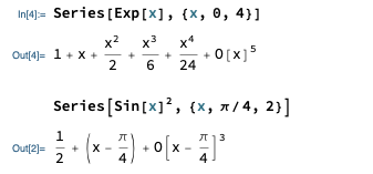
Going over the syntax: the first argument is the function you want to expand. The second argument consists of three things, collected in a list with {}: the name of the variable, the expansion point, and the maximum order that you want.
Example: another useful Taylor series
Find the Taylor series expansion of \( \ln(1+x) \) to third order about \( x=0 \).
If you're following along at home, try it yourself before you keep reading! This is the key piece that we'll need to go back and finish our projectiles with air resistance calculation.
Following the \( \epsilon \) version of the formula above, we can write this immediately as a Taylor series in \( x \) if we expand about \( 1 \). If we define \( f(u) = \ln(u) \) (changing variables to avoid confusion), then expanding about \( u_0 = 1 \) gives
\[ \begin{aligned} f(1+x) = f(1) + f'(1) x + \frac{1}{2} f''(1) x^2 + \frac{1}{3!} f'''(1) x^3 + ... \end{aligned} \]
(since \( u - u_0 = (1+x) - 1 = x \).) This is nice because it skips right to what we want, an expansion in the small quantity \( x \), but using the slightly simpler function \( \ln(u) \). If you instead took derivatives of \( \ln(1+x) \) in \( x \) directly, that's fine too - you'll get the same series.
Now we need the derivatives of \( \ln(u) \):
\[ \begin{aligned} f'(u) = \frac{1}{u} \\ f''(u) = -\frac{1}{u^2} \\ f'''(u) = \frac{2}{u^3} \end{aligned} \]
so \( f'(1) = 1 \), \( f''(1) = -1 \), and \( f'''(1) = 2 \). Finally, we plug back in to find:
\[ \begin{aligned} \ln(1+x) \approx x - \frac{1}{2} x^2 + \frac{1}{3} x^3 + ... \end{aligned} \]
Notice that this formula is also valid for negative values of \( x \), so if we want to expand \( \ln (1-x) \), we just flip the sign, i.e.
\[ \begin{aligned} \ln(1-x) \approx -\left(x + \frac{x^2}{2} + \frac{x^3}{3} + ... \right) \end{aligned} \]
Back to linear air resistance
This ends our important and lengthy math detour: let's finally go back and finish discussing projectile motion with linear air resistance. Our stopping point was the formula for the trajectory,
\[ \begin{aligned} y(x) = v_{\rm ter} \tau \ln \left( 1 - \frac{x}{\tau v_{x,0}} \right) + \frac{v_{y,0} + v_{\rm ter}}{v_{x,0}} x \end{aligned} \]
where \( v_{\rm ter} = mg/b \) and \( \tau = m/b \). We'd like to understand what happens as \( b \) becomes very small, where we should see this approach the usual "vacuum" result of parabolic motion. One option would be to plug the explicit \( b \)-dependence back in and series expand in that, but that will be messy for two reasons: there are \( b \)'s in several places, and \( b \) is a dimensionful quantity (units of force/speed = \( N \cdot s / m \), remember.)
Strictly speaking, we should never Taylor expand in quantities with units, because the whole idea is to expand in a small parameter, but if it has units we have to answer the question "small compared to what?" to see if our series is working or not.
Both problems can be solved by noticing that the combination
\[ \begin{aligned} \frac{x}{\tau v_{x,0}} = \frac{xb}{mv_{x,0}} \end{aligned} \]
is dimensionless, and definitely small as \( b \rightarrow 0 \) with everything else held fixed. This only appears in the logarithm, but the logarithm is the only thing we need to series expand anyway.
With that setup, let's apply our result for \( \ln(1+\epsilon) \) above, setting
\[ \begin{aligned} \epsilon = \frac{x}{\tau v_{x,0}}. \end{aligned} \]
We find:
\[ \begin{aligned} y(x) \approx v_{\rm ter} \tau \left[ -\frac{x}{\tau v_{x,0}} - \frac{x^2}{2\tau^2 v_{x,0}^2} - \frac{x^3}{3\tau^3 v_{x,0}^3} + ... \right] + \frac{v_{y,0} + v_{\rm ter}}{v_{x,0}} x \end{aligned} \]
We immediately spot that the very first term and the very last term are equal and opposite, so they cancel each other:
\[ \begin{aligned} y(x) \approx \frac{v_{y,0}}{v_{x,0}} x - v_{\rm ter} \tau \left[ \frac{x^2}{2\tau^2 v_{x,0}^2} + \frac{x^3}{3\tau^3 v_{x,0}^3} + ... \right] \end{aligned} \]
We'll continue to simplify this next time!