Picking up from last time: we series expanded the trajectory formula
\[ \begin{aligned} y(x) = v_{\rm ter} \tau \ln \left( 1 - \frac{x}{\tau v_{x,0}} \right) + \frac{v_{y,0} + v_{\rm ter}}{v_{x,0}} x \end{aligned} \]
in the small, dimensionless quantity \( x / (\tau v_{x,0}) \), finding the intermediate result:
\[ \begin{aligned} y(x) \approx \frac{v_{y,0}}{v_{x,0}} x - v_{\rm ter} \tau \left[ \frac{x^2}{2\tau^2 v_{x,0}^2} + \frac{x^3}{3\tau^3 v_{x,0}^3} + ... \right] \end{aligned} \]
As \( b \rightarrow 0 \), we know that \( v_{\rm ter} \) is becoming very large. This might make you worry about the \( v_{\rm ter} \tau \) appearing outside the square brackets, but remember that \( \tau \) is becoming large too, and we have some \( \tau \) factors in the denominator. In fact, we can go back to the definitions to notice that
\[ \begin{aligned} \frac{v_{\rm ter}}{\tau} = \frac{mg/b}{m/b} = g \end{aligned} \]
which we can use to continue simplifying:
\[ \begin{aligned} y(x) \approx \frac{v_{y,0}}{v_{x,0}} x - \frac{x^2 g}{2v_{x,0}^2} - \frac{x^3 g}{3 \tau v_{x,0}^3} + ... \end{aligned} \]
There's the quadratic term in \( x \), which no longer depends on anything to do with air resistance! In fact, now that we've simplified we can take \( b \rightarrow 0 \) completely, which will make \( \tau \rightarrow \infty \) and the third term vanish. This kills all of the higher terms in the expansion as well, leaving us with
\[ \begin{aligned} y_{\rm vac}(x) = \frac{v_{y,0}}{v_{x,0}} x - \frac{x^2 g}{2v_{x,0}^2}. \end{aligned} \]
This is, in fact, exactly the formula you'll find in your freshman physics textbook for projectile motion with no air resistance. Limit checked successfully!
Better still, we now have a nice approximate formula that we can use in cases where the air resistance is relatively small. (Explicitly, "small" in that we only consider values of \( x \ll \tau v_{x,0} \).) So long as this condition is satisfied, we see that we have a correction term for the vacuum trajectory which is of order \( x^3 \). For positive \( x \) this term is always negative, so the projectile will fall more quickly than it would in vacuum, matching our intuition that the drag force will slow down and hinder the projectile's motion.
As a last step, let's take our results and find the range \( R \), which is what Taylor focuses on in his discussion. The range is the value of \( x \) (not at zero) for which \( y=0 \). This is easily found for the vacuum solution:
\[ \begin{aligned} y_{\rm vac}(R) = 0 = \frac{v_{y,0}}{v_{x,0}} R - \frac{g}{2v_{x,0}^2} R^2 = R \left( \frac{v_{y,0}}{v_{x,0}} - \frac{g}{2v_{x,0}^2} R \right) \\ \Rightarrow R_{\rm vac} = \frac{2 v_{x,0} v_{y,0}}{g}. \end{aligned} \]
Now with drag turned on and including the cubic term, we get a quadratic equation:
\[ \begin{aligned} 0 = \frac{v_{y,0}}{v_{x,0}} R - \frac{g}{2v_{x,0}^2} R^2 - \frac{g}{3\tau v_{x,0}^3} R^3 + ... \end{aligned} \]
which, moving the \( R^2 \) term to the left and canceling one \( R \) off, we can rearrange as
\[ \begin{aligned} R = \frac{2 v_{x,0} v_{y,0}}{g} - \frac{2}{3\tau v_{x,0}} R^2. \end{aligned} \]
The second term here is proportional to the combination \( R/(\tau v_{x,0}) \), which is the small parameter we expanded in for the case of small drag. Thus, as \( b \rightarrow 0 \) the second term will go away and just leave the first term - which is just the vacuum result, once again.
However, we don't want to just completely throw away the second term - we want to know the leading correction due to the presence of air resistance. To do that, let's assume that the correction is small compared to the vacuum range: we write
\[ \begin{aligned} R = R_{\rm vac} + \delta R + ... \end{aligned} \]
where \( \delta R \ll R_{\rm vac} \). The (...) reminds us that this is implicitly an expansion in \( R/(\tau v_{x,0}) \), from which we're just keeping the first \( b \)-dependent term. We can plug this back in to our quadratic equation:
\[ \begin{aligned} R_{\rm vac} + \delta R = R_{\rm vac} - \frac{2}{3\tau v_{x,0}} (R_{\rm vac} + \delta R)^2 \end{aligned} \]
using the fact that we recognize the vacuum range as the first term on the right-hand side. Now, we can expand out the square on the right:
\[ \begin{aligned} \delta R = -\frac{2}{3\tau v_{x,0}} \left( R_{\rm vac}^2 + 2 R_{\rm vac} \delta R \right) \end{aligned} \]
where we throw away the \( (\delta R)^2 \) piece, because it's much smaller than everything else in the equation. (More properly, it's a higher-order piece in the expansion, so we shouldn't keep if it we've decided to work at first order.)
We can continue by solving for \( \delta R \), but we'll save a bit of work if we stop and think carefully about what terms we should keep. In particular, remember that \( R_{\rm vac} / (\tau v_{x,0}) \) is a small expansion parameter. Since the entire right-hand side is proportional to this small quantity, we should also throw away the \( R_{\rm vac} \delta R \) term, since it's also second-order as the air resistance goes to zero. That leaves us with the result:
\[ \begin{aligned} \delta R = -\frac{2R_{\rm vac}^2}{3\tau v_{x,0}} = -R_{\rm vac} \frac{4 v_{y,0}}{3 \tau g} = -R_{\rm vac} \frac{4 v_{y,0}}{3 v_{\rm ter}}. \end{aligned} \]
Plugging back in, we find our full result for the range at first order with air resistance,
\[ \begin{aligned} R \approx R_{\rm vac} \left( 1 - \frac{4 v_{y,0}}{3 v_{\rm ter}} \right). \end{aligned} \]
This is a small correction to the range so long as \( v_{y,0} \ll v_{\rm ter} \). If \( v_{y,0} \) is close to \( v_{\rm ter} \), this would be a large correction, but then we're also approaching the situation where our approximation is breaking down and we can't trust this result anymore!
I want to make one last point regarding series expansion and working to a certain order, before we move on to the next physics problem. Instead of doing the manipulations I did above and introducing the new variable \( \delta R \), it would have been perfectly valid to solve the quadratic equation for \( R \) instead,
\[ \begin{aligned} 0 = \frac{v_{y,0}}{v_{x,0}} - \frac{g}{2v_{x,0}^2} R - \frac{g}{3\tau v_{x,0}^3} R^2 + ... \end{aligned} \]
What if we just plug this in to the quadratic formula? The positive solution turns out to be:
\[ \begin{aligned} R = -\frac{3}{4} v_{x,0} \tau + \frac{\sqrt{3 \tau} v_{x,0}}{4g} \sqrt{3g^2 \tau + 16g v_{y,0}}. \end{aligned} \]
This looks messy, and also doesn't look even remotely like the result we found above! Why is this equation so different? The short answer is that we have to remember that we're working with a series expansion as \( b \rightarrow 0 \), and therefore in \( \tau \rightarrow \infty \). So we have to expand out functions like square roots involving \( \tau \), and just keep the leading terms, or else we're fooling ourselves!
I won't try to do this by hand in class, because the algebra is a little messy, but we can use Mathematica to carry out the expansion for us at \( \tau = \infty \):
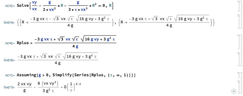
Tricks of the trade: the Assuming[] statement makes the answer look nicer, otherwise you'll end up with things like \( \sqrt{g^2} / g \) which Mathematica will refuse to cancel off, assuming \( g \) might be negative. Also, notice that we can series expand directly at infinity: type Esc-i-n-f-Esc as a shortcut to write the infinity symbol. If you were doing this by hand, you would instead want to define \( \epsilon = 1/\tau \) and then expand at \( \epsilon = 0 \).
Having worked out the algebra, we have our result, which we can write most clearly by factoring out the vacuum range:
\[ \begin{aligned} R = \frac{2v_{x,0} v_{y,0}}{g} \left( 1 - \frac{4v_{y,0}}{3g\tau} \right) = R_{\rm vac} \left( 1 - \frac{4v_{y,0}}{3v_{\rm ter}} \right). \end{aligned} \]
Quadratic drag
Let's turn to purely quadratic air resistance now:
\[ \begin{aligned} \vec{f}(v) = -cv^2 \hat{v} \end{aligned} \]
As a reminder, this will be an accurate model for situations in which \( cv^2 \gg bv \), or equivalently when the Reynolds number \( R = D \rho v / \eta \) is much larger than 1. For most everyday objects moving at normal speeds, \( R \gg 1 \) and the quadratic model is the one which applies. (However, as I'll emphasize again later, if \( v \) is too small the quadratic drag is vanishing, so we have to be careful if our object is coming to a stop!)
Following the linear case study, I'll start with horizontal motion. For an object moving purely in the \( +\hat{x} \) direction subject to quadratic drag, and no other forces, we have the equation of motion
\[ \begin{aligned} m \ddot{x} = -c \dot{x}^2. \end{aligned} \]
Written in terms of \( v_x \) this is a separable first-order ODE; in fact, it's one we solved as an exercise back when we were talking about ODEs in general. The solution we found was
\[ \begin{aligned} v(t) = \frac{v_0}{1 + \frac{cv_0}{m} t} = \frac{v_0}{1 + t/\tau_c}, \end{aligned} \]
defining the quadratic natural time
\[ \begin{aligned} \tau_c = \frac{m}{cv_0}. \end{aligned} \]
(Notation break from Taylor: he just calls this \( \tau \) as well. I wanted to label it clearly as different from the linear version.)
Checking units is a good habit, so let's make sure this is indeed a time. \( c \) must have units of force over speed squared, or \( N \cdot s^2 / m^2 \), which means \( cv_0 \) is in \( N \cdot s / m = kg / s \) using the definition of a Newton (which is easy to remember since \( \vec{F} = m\vec{a} \).) The mass up top cancels the \( kg \), leaving \( s \), so indeed this is a time. Specifically, we see that \( t=\tau_c \) is the time at which the initial speed is halved,
\[ \begin{aligned} v(\tau_c) = \frac{v_0}{2}. \end{aligned} \]
To avoid confusion, notice that this is not the same as a half-life that would appear in radioactive decay! In particular, \( v(2\tau) = v_0 / 3 \), whereas if we waited for two half-lives we would expect to have \( 1/2^2 = 1/4 \) of our initial sample remaining. The difference is that our solution \( v(t) \) is not exponential in time, but instead dies off much more slowly as \( t \rightarrow \infty \).
What about position as a function of time? We can obtain that just by integrating once, as always:
\[ \begin{aligned} x(t) = x_0 + \int_0^t dt' v(t') \\ = x_0 + \int_0^t dt' \frac{v_0}{1+t'/\tau_c} \\ = x_0 + v_0 \tau_c \ln \left( 1 + \frac{t}{\tau_c} \right). \end{aligned} \]
Here are a couple of sketches of the time dependence, before we discuss further:
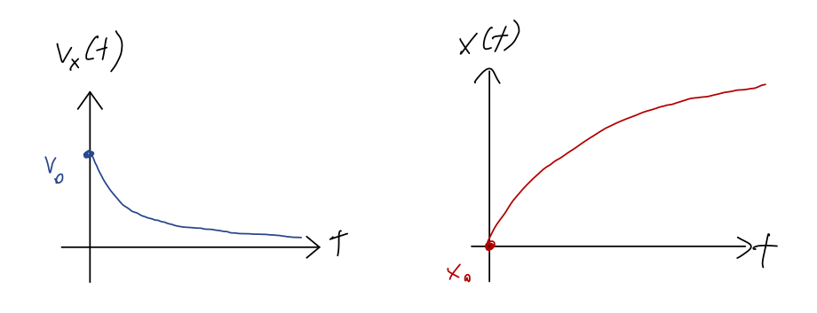
You may remember in the linear drag case that the \( x \) position approached a finite asymptotic value \( x_\infty \) as our object came to a stop. That's not true in this case: the logarithm actually never stops growing with \( t \), so \( \lim_{t \rightarrow \infty} x(t) = \infty \)! This is because as we already noted, in the quadratic case, the speed \( v(t) \) decreases more slowly with time.
This might seem really weird, because we seem to be concluding that a moving object under the effects of quadratic drag can travel infinitely far without stopping - and this is the case that is appropriate for everyday objects! The key point to remember is that this model will inevitably become invalid when \( v(t) \) becomes small enough: as the quadratic drag force becomes smaller, eventually some other force (linear drag, or friction) will be large enough that we can't ignore it anymore.
Taylor gives the nice example of a person riding a bicycle, coasting to a stop from a fairly high speed. Our quadratic drag model for \( x(t) \) will describe this motion well for a while, but eventually as the bicycle slows down, ordinary friction between the wheels and the ground will become large enough to notice, bringing it to a stop in a finite distance. (Linear drag could do the same thing, but it so happens that friction is stronger for the bicycle case.)
Vertical motion with quadratic drag
Now let's look at vertical motion, which means turning on gravity. This time, we have to be really careful about minus signs! Let's think it through to make sure we find the right equation of motion.
Clicker Question
Which is the correct equation of motion to describe both cases, \( v_y > 0 \) and \( v_y < 0 \)?
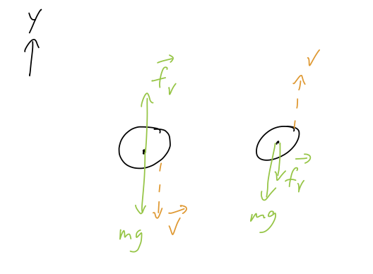
(The sign function \( {\rm sgn}(x) \) is equal to \( +1 \) if \( x>0 \), and \( -1 \) if \( x<0 \).)
A. \( \dot{v}_y = -g - \frac{c}{m} v_y^2 \)
B. \( \dot{v}_y = -g + \frac{c}{m} v_y^2 \)
C. \( \dot{v}_y = -g - {\rm sgn}(v_y) \frac{c}{m} v_y^2 \)
D. \( \dot{v}_y = -g + {\rm sgn}(v_y) \frac{c}{m} v_y^2 \)
Answer: C
The simplest way to work this out is to start by staring at the provided free-body diagram. We see that (as in the linear case) the drag force should be positive if \( v_y \) is negative, and vice-versa. However, unlike the linear case, the \( v_y^2 \) is always positive - which is why we need the sign function to help fix things!
Comparing C with D, when \( v_y < 0 \) then the sign function \( {\rm sgn}(v_y) = -1 \), so to end up with a positive drag force we need one more minus sign, leading us to answer C.