Finishing the example from last time: we found the solution
\[ \begin{aligned} v_y(t) = -v_{\rm ter,c} \tanh \left( \frac{t}{\tau} \right) \end{aligned} \]
with \( v_{\rm ter, c} = 3.8 \) m/s and \( \tau = 2.6 \) s. Furthermore, we decided to use a series expansion instead of working with \( \tanh \) directly, finding the result
\[ \begin{aligned} \tanh(x) = (x+...) (1 - x + ...) = x + \mathcal{O}(x^3) \end{aligned} \]
(with no \( \mathcal{O}(x^2) \) terms because \( \tanh \) is odd.) From this expansion, we have
\[ \begin{aligned} v_y(t) \approx -v_{\rm ter,c} \frac{t}{\tau} \end{aligned} \]
and then
\[ \begin{aligned} y(t) \approx \int_0^t\ v_y(t')\ dt' = -\frac{v_{\rm ter,c} t^2}{2\tau} \\ \Rightarrow t = \sqrt{\frac{2h\tau}{v_{\rm ter,c}}} \end{aligned} \]
where \( h \) is the drop height. Plugging in numbers gives \( t \approx 0.45 \) s.
Now, the final question: do I trust the series expansion result?
Clicker Question
Do we trust the series expansion result, given that \( t \approx 0.45 \) s and \( \tau = 2.6 \) s?
\[ \begin{aligned} v_y(t) = -v_{\rm ter, c} \tanh \left( \frac{t}{\tau} \right) \approx -v_{\rm ter, c} \frac{t}{\tau} \end{aligned} \]
A. No, the error might be very large because we integrated over \( t \). We need the next term!
B. Sort of, the truncation error is of order \( t/\tau \approx 1/5 \), or 20% - we have a rough idea at least.
C. Yes, the truncation error is of order \( t^2 / \tau^2 \approx 1 / 25 \), or 4% - good enough for a bar argument.
D. Definitely, the truncation error is of order \( t^3 / \tau^3 \approx 1/125 \), or less than 1% - precise enough that other sources of error are probably bigger!
Answer: C
This is a question about error due to series expansion, usually we would state the condition to use the expansion as "\( t \ll \tau \)". But let's be more precise. By using a series expansion, the error we're making is roughly the size of the first missing term in the expansion, which is proportional to \( (t/\tau)^3 \). If we had kept that term, our formula for \( v_y(t) \) would have been
\[ \begin{aligned} v_y(t) \approx -v_{\rm ter,c} \frac{t}{\tau} \left(1 + K \frac{t^2}{\tau^2} \right), \end{aligned} \]
where to figure out \( K \) we'd have to compute the Taylor expansion out to third order. If we really want to be careful, we can do just that, but instead let's assume \( K \) is not too far from 1. Then what matters is the size of \( t2/\tau2 \), which is
\[ \begin{aligned} \frac{t^2}{\tau^2} \approx 0.03. \end{aligned} \]
So, up to the size of whatever the number \( K \) turns out to be, we're making an error of around 3% in \( v_y(t) \) by using the first-order series expansion. The first observation we can make is that since this is much smaller than 1, we don't have to worry about convergence of the series, i.e. the first-order answer is a good initial guess.
Beyond that, do we need to go find the next term in the expansion? If I'm just observing this process happening by eye, then probably not; I don't think a human observer would easily notice differences on the order of a few hundredths of a second. On the other hand, if I want to know the answer to within 1% accuracy - maybe if I want to make measurements of this kind of motion to work backwards and calculate the density of the beer, for example - then I do need to keep the next term in the series.
To summarize: the order at which we stop is always found by the accuracy at which we need the answer; and (as long as the series converges!) we can always get better accuracy by continuing the expansion to the next order.
Projectiles with quadratic resistance; linear + quadratic resistance
At this point, the obvious next step would be to try to put our solutions together to study projectile motion with quadratic drag. Unfortunately, there's an obstacle to doing this that wasn't present in the linear case, which we can see if we go back to the vector form of Newton's second law. In the linear case, we have
\[ \begin{aligned} \vec{F} = m\dot{\vec{v}} = m\vec{g} - bv \hat{v} = m\vec{g} - b\vec{v}. \end{aligned} \]
This splits cleanly into two separate equations for \( v_x \) and \( v_y \), because only \( \vec{v} \) appears on both sides. However, in the quadratic case, the general equation is
\[ \begin{aligned} m\dot{\vec{v}} = m\vec{g} - cv^2 \hat{v} = m\vec{g} - cv \vec{v}. \end{aligned} \]
This almost splits up in the same way, but we have an extra factor of \( v \), which is the overall speed. If we write this full equation out in components, we find
\[ \begin{aligned} \dot{v}_x = -\frac{c}{m} \sqrt{v_x^2 + v_y^2} v_x \\ \dot{v}_y = -g - \frac{c}{m} \sqrt{v_x^2 + v_y^2} v_y. \end{aligned} \]
These are non-linear ODEs, but even worse they're coupled ODEs, meaning that we have to solve them simultaneously because each equation depends on the other unknown velocity component. In fact, the only way we can deal with these more complicated equations is to solve them numerically. Taylor talks a little bit about this, but I'll let you read his example and will not say any more here.
We run into a similar problem if we try to solve the general case of having both linear and quadratic drag forces,
\[ \begin{aligned} m\dot{\vec{v}} = m\vec{g} - b\vec{v} - cv \vec{v} \end{aligned} \]
which would be required when the Reynolds number is close to 1. It is actually possible to solve the horizontal- and vertical-motion cases analytically here, but those full solutions won't show off anything new and interesting in terms of either physics or math, so we'll skip over them. The full study of projectile motion with both terms can only be done numerically due to the quadratic term.
Momentum and conservation laws
Our next big physics topic is going to be momentum. Although we've sort of been ignoring it when solving problems, the concept of momentum is central to all three of Newton's laws, and in fact the way we write the second law,
\[ \begin{aligned} \vec{F} = m \ddot{\vec{r}}, \end{aligned} \]
is actually not always correct! The most general correct form of Newton's second law is the one stated in terms of momentum,
\[ \begin{aligned} \vec{F} = \dot{\vec{p}}. \end{aligned} \]
This is the version that applies when we extend mechanics to include special relativity. It's also the version that applies in the case that \( m \) depends on time - the most important example of such a system is a rocket, which we'll be studying in detail.
Momentum is also a really useful concept because it obeys a conservation law, which you've certainly learned in intro physics and which we'll re-derive next. The general idea of a conservation law is simple: if \( C \) is some property of a physical system, then we say that \( C \) is conserved if
\[ \begin{aligned} \frac{dC}{dt} = 0, \end{aligned} \]
i.e. if \( C \) doesn't change with time. This is a simple but really powerful observation! Having a conservation law lets us do several useful things:
- If we know the starting and ending points of our system, we can calculate \( C_{\rm initial} \) and \( C_{\rm final} \), and they must be equal.
- If there are parts within \( C \) that do depend on time, then setting \( dC/dt = 0 \) can give us a useful and relatively simple differential equation relating them.
- A conservation law can give us powerful qualitative insights about how different parts of a physical system interact with each other and with the outside world. For example, energy conservation means that there is no such thing as "free energy" - if a black box is producing mechanical energy, it has to be transferred from somewhere!
There is an even deeper connection between conservation laws and symmetries, which are ways in which you can change an experiment without changing the result. Probably the most important symmetry in nature, and the reason that science can work at all, is known as time translation symmetry: the fact that if you wait a little while after an experiment and then repeat it (being careful to reset the initial conditions), the outcome will be the same. It turns out that this all-important symmetry actually leads to one of the most important conservation laws, conservation of energy. Unfortunately, the framework to prove that is something you won't see until next semester, so you'll have to stick around to see it!
Conservation of linear momentum
Now let's dig into the first important conservation law we'll discuss, conservation of linear momentum. I'll state it first:
"For any physical system which is subject to zero net external force, the total combined linear momentum \( \vec{P} \) of all objects in that system satisfies \( d\vec{P}/dt = 0 \)."
This can be thought of an extension of Newton's second law, since \( \vec{F} = \dot{\vec{p}} \) immediately tells us that for a single point mass, its momentum is conserved with no force acting on it. The more subtle point is that we're claiming this is true even for a system of masses. So the second-law approach will only work if we can also show that \( \vec{F}_{\rm ext} \), the net external force, is equal to \( \dot{\vec{P}} \), the rate of change of total momentum.
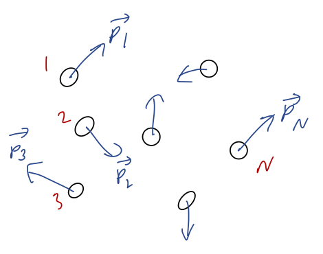
To work this out in general, we'll say that we have a collection of \( N \) point masses, with masses \( m_1, m_2, ..., m_N \). They can all move independently, so we'll also have to keep track of \( N \) momentum vectors \( \vec{p}_1, \vec{p}_2, ..., \vec{p}_N \). (Likewise there are \( N \) position vectors \( \vec{r}_1, ..., \vec{r}_N \), but we won't need to refer to them for present purposes.)
Let's start by just focusing on the first two masses, 1 and 2. To be completely general, there can be forces acting between these two particles in either direction. (Our collection could be a liquid, or a solid, in which case we have bonding forces; it could be a bunch of asteroids, which would have a gravitational force; it could be a collection of electric charges...) We can divide up the net force on each object to single out that piece:
\[ \begin{aligned} \vec{F}_1 = \vec{F}_{12} + \vec{F}_{1,\rm{ext}} \\ \vec{F}_2 = \vec{F}_{21} + \vec{F}_{2,\rm{ext}} \end{aligned} \]
where \( \vec{F}1 \) is the net force acting on mass 1, \( \vec{F}{12} \) can be read as "the force on mass 1 by mass 2", and \( \vec{F}_{1,\rm{ext}} \) just represents all other forces external to the mass 1 - mass 2 system.
Now, we know that Newton's second law will hold for each of our two masses, so
\[ \begin{aligned} \vec{F}_1 = \frac{d\vec{p}_1}{dt},\ \ \vec{F}_2 = \frac{d\vec{p}_2}{dt}. \end{aligned} \]
This means that if we define the total momentum \( \vec{P_{12}} \equiv \vec{p}_1 + \vec{p}_2 \), then
\[ \begin{aligned} \frac{d\vec{P}_{12}}{dt} = \vec{F}_1 + \vec{F}_2 = \vec{F}_{1,\rm{outside}} + \vec{F}_{2,\rm{ext}} + \vec{F}_{12} + \vec{F}_{21}. \end{aligned} \]
But now, we can call on Newton's third law: the net forces between objects 1 and 2 must be equal and opposite, \( \vec{F}{21} = -\vec{F}{12} \). This means that the last two terms above cancel, and we just have
\[ \begin{aligned} \frac{d\vec{P}_{12}}{dt} = \sum_{\alpha=1}^2 \vec{F}_{\alpha,\rm{ext}} = \vec{F}_{\rm net, ext}. \end{aligned} \]
(On the last line I used summation notation to rewrite the sum of two outside forces, and then combined them into a single net force. We'll be using sums a lot when we move past two masses!) So for two masses in isolation, we find that the combination of Newton's second and third laws allows us to conclude that the combined momentum satisfies Newton's second law, in terms of the outside forces acting on the pair; the momentum change due to the internal forces cancelled out in the sum.
Seeing that it works in the simple case, let's move on to the full set of \( N \) particles. The manipulations we need to do will be similar, but we'll have to keep track of all of the pieces. Let's start with mass 1 again, singling out the force on it due to each other particle:
\[ \begin{aligned} \vec{F}_1 = \vec{F}_{12} + \vec{F}_{13} + ... + \vec{F}_{1N} + \vec{F}_{1,\rm{ext}} \\ = \sum_{\alpha=2}^N \vec{F}_{1\alpha} + \vec{F}_{1,\rm{ext}} \end{aligned} \]
using summation notation to write this more compactly. Similarly for the second mass,
\[ \begin{aligned} \vec{F}_2 = \vec{F}_{21} + \vec{F}_{23} + ... + \vec{F}_{2N} + \vec{F}_{2,\rm{ext}} \\ = \sum_{\alpha \neq 2} \vec{F}_{2\alpha} + \vec{F}_{2,\rm{ext}} \end{aligned} \]
where we're adopting a new notation for the sum, which means "sum over all possible values of \( \alpha \), except for \( \alpha = 2 \)" - which is missing because mass 2 can't exert any force on itself. (In this notation it's implied that \( \alpha \) runs from 1 to \( N \), instead of explicitly written on the symbol.) Seeing the pattern, we can write for an arbitrary mass \( \beta \)
\[ \begin{aligned} \vec{F}_\beta = \sum_{\alpha \neq \beta} \vec{F}_{\beta \alpha} + \vec{F}_{\beta, \rm{ext}}. \end{aligned} \]
Newton's second law tells us that \( \vec{F}\beta = d\vec{p}\beta/dt \). As before, our next step is to put together the total momentum of the system,
\[ \begin{aligned} \vec{P} = \sum_\beta \vec{p}_\beta. \end{aligned} \]
Now we take the time derivative and apply Newton's second law:
\[ \begin{aligned} \frac{d\vec{P}}{dt} = \sum_\beta \frac{d\vec{p}_\beta}{dt} = \sum_\beta \vec{F}_\beta \\ = \sum_\beta \left( \sum_{\alpha \neq \beta} \vec{F}_{\beta \alpha} + \vec{F}_{\beta, \rm{ext}} \right). \end{aligned} \]
Next time: we finish the derivation, and see some practical examples.