Finishing up the two-stage rocket from last time, here's the setup again:
Rocket A is simple rocket with a fuel-to-mass ratio of \( m_{A,F} / m_{A,E} = 25 \). Rocket B is a two-stage rocket, which means it's two rockets stuck together: both stage 1 and stage 2 have a fuel-to-mass ratio of \( m_{B1,F} / m_{B1,E} = m_{B2,F} / m_{B2,E} = 10 \). Stage 2 is also about 5 times lighter than stage 1, i.e. \( m_{B1,E} / m_{B2,E} = 5 \).
We found the \( \Delta v \) for rocket A to be:
\[ \begin{aligned} (\Delta v)_A = |v_{\rm exh}| \log \left(1 + \frac{m_{A,F}}{m_{A,E}} \right) \\ = |v_{\rm exh}| \log \left(1 + 25 \right) = 8.1\ {\rm km} / {\rm s} \end{aligned} \]
For the two-stage rocket, we have to be more careful what masses we plug in. Let's working in units of the mass of the empty second stage, \( m_{B2,E} \equiv m \), since this is the lightest mass in the problem. In these units, we have for example the empty first stage \( m_{B1,E} = 5m \).
Clicker Question
In units of \( m = m_{B2,E} \), what are the correct fuel (\( m_F \)) and empty (\( m_E \)) masses for the first-stage burn of the two-stage rocket?
A. \( m_F = 50m, m_E = 5m \)
B. \( m_F = 50m, m_E = 16m \)
C. \( m_F = 60m, m_E = 6m \)
D. \( m_F = 60m, m_E = 11m \)
E. \( m_F = 60m, m_E = 16m \)
Answer: B
We are told that the fuel-to-mass ratios for both of the two stages are 10. So since (from above) the empty masses of the stages are \( m_{B2,E} = m \) and \( m_{B1,E} = 5m \), we have \( m_{B2, F} = 10m \) and \( m_{B1, F} = 50m \).
For the first stage, only the mass of the burned fuel matters. So \( m_F = 50m \), the fuel in the first stage alone. For the "empty" mass, however, we need to be more careful: the "empty" first stage includes the mass of the second stage, which is being carried as cargo! This includes the second-stage fuel, which hasn't been burned yet. Thus, the mass after the burn is
\[ \begin{aligned} m_E = m_{B1,E} + m_{B2,F} + m_{B2,E} = 5m + 10m + m = 16m \end{aligned} \]
giving answer B.
Thus, after the first-stage burn, we have
\[ \begin{aligned} (\Delta v)_{B1} = |v_{\rm exh}| \log \left(1 + \frac{50}{16} \right) = 3.5\ {\rm km} / {\rm s} \end{aligned} \]
Now we discard the first stage and just consider the second stage alone, which is much easier to plug in for:
\[ \begin{aligned} (\Delta v)_{B2} = |v_{\rm exh}| \log \left(1 + 10\right) = 6.0\ {\rm km} / {\rm s} \end{aligned} \]
So in total, the second rocket achieves
\[ \begin{aligned} (\Delta v)_B = 9.5\ {\rm km}/{\rm s}, \end{aligned} \]
somewhat better than rocket A - despite the fact that the individual stages had a much lower fuel-to-mass ratio! Qualitatively, this makes sense: if we can dump some of the mass of our rocket partway through, then the fuel-to-mass ratio at that point is immediately improved. (After the first-stage burn but before separation, our fuel-to-mass ratio is all the way down to 1.7.)
By the way, 25 to 1 is generally considered about the best possible ratio for a single rocket stage, based on available technology for both rocket fuels and engineering the rocket itself. The ratio of 5 in mass between the two stages is taken from SpaceX's Falcon 9 rocket, but the real Falcon 9 has much better single-stage performance, with 18:1 for the first stage and 25:1 for the second. This gives the Falcon 9 an approximate \( \Delta v \) of 12.1 km/s (before including a payload) - large enough that we can start thinking about escaping the Earth completely and going elsewhere in the Solar system (like Mars!)
Angular momentum
Before we move on to energy, let's have a brief look at angular momentum. The definition of angular momentum is
\[ \begin{aligned} \vec{\ell} = \vec{r} \times \vec{p} = m\vec{r} \times \dot{\vec{r}} \end{aligned} \]
for a point mass. You should have seen the cross product before, but this is a good point to remind you of some definitions.
Unlike the dot product, the cross product \( \vec{a} \times \vec{b} \) gives us another vector instead of a number, and in particular \( \vec{a} \times \vec{b} \) by definition is perpendicular to both \( \vec{a} \) and \( \vec{b} \). The magnitude of the cross product is
\[ \begin{aligned} |\vec{a} \times \vec{b}| = ab \sin \theta \end{aligned} \]
behaving in the opposite way to the dot product; in particular, notice that \( |\vec{a} \times \vec{a}| \) is always zero.
Now, given two different vectors \( \vec{a} \) and \( \vec{b} \), there is a unique plane containing both of them; the direction of the cross product \( \vec{a} \times \vec{b} \) is then perpendicular to that plane. However, this isn't quite enough information, because \( -\vec{a} \times \vec{b} \) is also perpendicular to the plane!
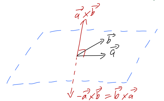
Deciding which of these two vectors to call the positive cross product is a choice of convention - which means it's an arbitrary choice that we can make once, but then we have to keep that choice consistent. We will follow the standard physics convention, which is the right-hand rule: if you hold out your right hand with the thumb pointing in the direction of \( \vec{A} \) and your fingers in the direction of \( \vec{B} \), then your palm points in the direction of \( \vec{A} \times \vec{B} \). Try it with my diagram above!
The right-hand rule also fixes an ambiguity in our rectangular coordinates, which is that we could have picked either of these sets of axes:
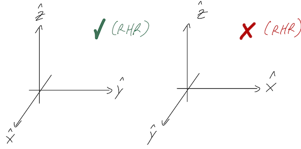
We always define our rectangular coordinates so that positive \( \hat{z} \) is a right-hand rule cross product of \( \hat{x} \) with \( \hat{y} \). In other words, the directions of our rectangular unit vectors always satisfy:
\[ \begin{aligned} \hat{x} \times \hat{y} = \hat{z} \\ \hat{y} \times \hat{z} = \hat{x} \\ \hat{z} \times \hat{x} = \hat{y}. \end{aligned} \]
This is only one choice of convention, and not three; the first equation actually forces the other two to be true. An easy way to remember all three of these at once is to notice that they are all cyclic permutations: if you shift every vector to the left one spot, wrapping back around to the right at the left end, then you get the next formula.
There is a general, mechanical formula for the cross product in rectangular components, using a three-by-three matrix determinant:
\[ \begin{aligned} \vec{a} \times \vec{b} = \left|\begin{array}{ccc} \hat{x}&\hat{y}&\hat{z}\\ a_x&a_y&a_z\\ b_x&b_y&b_z\end{array}\right| \\ = (a_y b_z - a_z b_y) \hat{x} - (a_x b_z - a_z b_x) \hat{y} + (a_x b_y - a_y b_x) \hat{z}. \end{aligned} \]
We will use this a couple of times this semester, and you'll see lots more of it next semester in classical mechanics 2.
Now back to angular momentum, \( \vec{\ell} \equiv \vec{r} \times \vec{p} \). It's very important to stress that, unlike linear momentum, this depends strongly on what the origin of our coordinate system is! Consider the following example: we have a 1 kg mass moving in a straight line at \( v = 2 \) m/s. Here's a sketch with two possible coordinate systems:
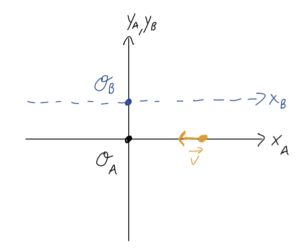
The linear momentum of the particle is the same in both coordinate systems, \( \vec{p} = (-2,0,0)\ {\rm kg} \cdot {\rm m} / {\rm s} \). However, the angular momentum is different:
\[ \begin{aligned} \vec{\ell}_A = \vec{r}_A \times \vec{p} = (4,0,0) \times (-2, 0, 0) = (0,0,0)\ {\rm kg} \cdot {\rm m}^2 / {\rm s} \\ \vec{\ell}_B = \vec{r}_B \times \vec{p} = (4, -2, 0) \times (-2, 0, 0) = (0,0,-4)\ {\rm kg} \cdot {\rm m}^2 / {\rm s} \end{aligned} \]
(check the direction with the right-hand rule!) Of course, this isn't really a fundamental difference: if I set up a third coordinate system with origin \( \mathcal{O}_C \) which is moving to the left at 2 m/s, then the linear momentum will change to \( \vec{p}_C = (0,0,0) \). Momentum is something that we define to make sense of a physical system, but all that really matters is the actual motion is the same no matter what coordinates we choose. (I stress this point here because it often catches people off-guard that angular momentum can change even if your coordinates aren't moving.)
In the presence of forces, \( \vec{p} \) will change, and therefore \( \vec{L} \) can also be changed by forces. To see exactly how, we just take the time derivative:
\[ \begin{aligned} \frac{d\vec{\ell}}{dt} = m\frac{d}{dt} \left(\vec{r} \times \dot{\vec{r}} \right) \\ = m \dot{\vec{r}} \times \dot{\vec{r}} + m \vec{r} \times \ddot{\vec{r}} \\ = \vec{r} \times \vec{F}, \end{aligned} \]
where on the last line the first term vanished since it's the cross product of a vector with itself, and in the second term we plugged in Newton's second law. This cross product of distance and force is called the torque,
\[ \begin{aligned} \vec{\Gamma} \equiv \vec{r} \times \vec{F}. \end{aligned} \]
(Some references will use \( \tau \) instead of \( \Gamma \) for torque, so beware.) This gives us a rotational version of Newton's second law,
\[ \begin{aligned} \vec{\Gamma} = \frac{d\vec{\ell}}{dt}. \end{aligned} \]
Conservation of angular momentum
We can identify a new conservation law from the last equation we wrote above: if there is no net torque on a point mass, \( \vec{\Gamma} = 0 \), then angular momentum is conserved - \( d\vec{\ell} / dt = 0 \). Note that this can be true even if there is a net force, as long as \( \vec{r} \times \vec{F} = 0 \).
Of course, this isn't very useful for a single point mass! There are not many situations where there is a net force but no torque for the entire motion of a single particle, just because \( \vec{r} \) will generally change with time. The good news is that like conservation of linear momentum, this law also applies to collections of masses. Breaking out our trusty set of \( N \) point masses \( {m_\alpha } \), it can be shown that if we define the total angular momentum
\[ \begin{aligned} \vec{L} \equiv \sum_{\alpha=1}^N \ell_\alpha, \end{aligned} \]
then \( \dot{\vec{L}} = 0 \) if the net external torque is zero, and more generally,
\[ \begin{aligned} \vec{\Gamma}_{\rm ext} = \frac{d\vec{L}}{dt}. \end{aligned} \]
(I am not going to do the proof in class - it's another round of sums, but this time with cross products added in. Taylor shows this result in chapter 3.5, and I encourage you to have a look.)
As with conservation of linear momentum, a nice application of this conservation law is learning things about horribly complicated systems, so long as they have no external torques acting on them. The formation of the solar system, for example, was a horribly messy and complicated process spanning billions of years. However, from the simple fact that the planets currently have a net angular momentum (all of the orbits go the same way, which is the same way the Sun is spinning!), we know that whatever primordial structure the solar system formed from must have been spinning, and we can even relate its rotational speed to its size!
This is especially useful in combination with the center of mass (CM)! It turns out that for any extended object, we can decompose its motion into two parts: the motion of the CM itself, treating it like a point particle, and then rotation of the object about the CM. The latter subject is fairly complicated, but you'll see it worked out in detail next semester, and it's much, much easier to study rotation using the CM of an object instead of using an arbitrary set of coordinates.
There are a couple of immediate applications that we could try to work through - Taylor shows a few examples, including a version of Kepler's second law. But these are specialized examples, especially the planetary motion one, and I think it's better to put them off until you're really prepared to tackle the problem of rotation and angular momentum in full. So we'll end the chapter here.