Before we can continue our study of work and kinetic energy, we have to deal with an important question: how do we evaluate the integral for work in general? Having another look at it:
\[ \begin{aligned} W_{\rm net} = \int_{\vec{r}_1}^{\vec{r}_2} \vec{F}_{\rm net} \cdot d\vec{r} \end{aligned} \]
How do we interpret this integral, where the integration variable is a vector? The best way to understand what this expression means is to go back to the infinitesmal picture for \( dW \), and imagine building up the whole integral by just stringing together infinitesmal pieces:
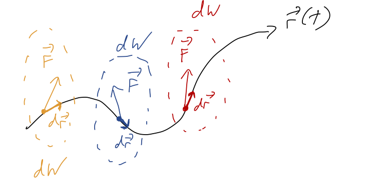
So the integral for \( W \) is a sum along the path traced out by \( \vec{r} \).,
\[ \begin{aligned} W = \sum_i dW_i \rightarrow \int dW \end{aligned} \]
where the sum becomes an integral as we make our steps along the trajectory \( d\vec{r} \) smaller and smaller. Notice that this is not the "area under the curve" or anything related to it; we're summing up the dot products \( \vec{F}_{\rm net} \cdot d\vec{r} \) as we follow the curve. This is an example of a line integral.
There's one special case where we already know how to do the integral: if the motion is one-dimensional. For one-dimensional motion, all vectors have only one component, so the dot product is trivial. If we call our single direction \( x \), then
\[ \begin{aligned} W_{1d} = \int_{x_1}^{x_2} \vec{F}_{\rm net}(x) \cdot d\vec{x} \end{aligned} \]
(I'm keeping the dot product notation to remind us that the directions still matter in one dimension, so we can get minus signs here.)
Now let's pick a concrete example in two dimensions to see how things get tricky. Suppose that we have a constant force of the form
\[ \begin{aligned} \vec{F} = Fx\hat{x} + 2F\hat{y}, \end{aligned} \]
and we'd like to compute the work from \( \vec{r}_1 = (0,0) \) to \( \vec{r}_2 = (2,1) \). How do we interpret the vector differential \( d\vec{r} \)? We already know that derivatives of vectors are simple to evaluate: we just take the derivative of each component. Similarly, \( d\vec{r} \) just means we have a differential length in each component. In Cartesian coordinates,
\[ \begin{aligned} d\vec{r} = dx \hat{x} + dy \hat{y} + dz \hat{z}. \end{aligned} \]
So in our example, we can evaluate the dot product to find
\[ \begin{aligned} W = \int_{\vec{r}_1}^{\vec{r}_2} (Fx dx + 2F dy). \end{aligned} \]
The appearance of two differentials at once, \( dx \) and \( dy \), signals that we can't just evaluate this integral normally yet. More importantly, we have to specify one more thing not written down, which is the path along which we want to evaluate this integral. This is one of the sloppy things about this notation, although it's used commonly: there are infinitely many ways to get from \( \vec{r}_1 \) to \( \vec{r}_2 \)!
Notice that these are directed paths, hence the arrows; just like a regular integral, if we go backwards (reverse the limits of integration so we move from \( \vec{r}_2 \) to \( \vec{r}_1 \)), then we get an extra minus sign.
In math books, the integral will often be written instead as
\[ \begin{aligned} W = \int_\mathcal{C} \vec{F} \cdot d\vec{r}, \end{aligned} \]
where \( \mathcal{C} \) denotes a curve - the entire path we take, along with its endpoints. In physics applications, when we do the work integral, the curve is always \( \vec{r}(t) \), the trajectory followed by our point mass.
Let's pick one of the curves above and try to evaluate the integral. I'll start with the straight line path, \( \mathcal{C}_1 \). If we think about it for a moment, the way a path is mathematically defined is an equation relating our coordinates to each other. In this case, we can write simply
\[ \begin{aligned} y = \frac{1}{2}x \end{aligned} \]
along \( \mathcal{C}_1 \). This relationship is true as long as we follow the curve. But we can use this to collapse our two differentials together: we have
\[ \begin{aligned} dx = 2dy \end{aligned} \]
so we can rewrite the line integral as
\[ \begin{aligned} W_1 = \int_{\mathcal{C}_1} (F xdx + 2F dy) \\ = \int_0^1 (F (2y) (2 dy) + 2F dy) \\ = F \left( \left. 4 \frac{y^2}{2} \right|_0^1 + \left. 2y \right|_0^1 \right) \\ = 4F. \end{aligned} \]
This shows the basic idea of evaluating a line integral: although it looks like it has multiple coordinate differentials in it, when we move along a specific line, we can relate our coordinates together and collapse down to a single differential. Then we just have a normal integral to do! (It will always be a single integral, because a line is one-dimensional; we can always describe the distance along a line using a single number, whether the line is curved or not.)
An important feature of this method is that the way in which we collapse our multiple coordinates down to one is not unique. For example, we could have replaced \( dy \) instead of \( dx \), and we'll get the same answer:
\[ \begin{aligned} W_1 = \int_{\mathcal{C}_1} (Fx dx + 2F (dx/2)) \\ = \int_0^2\ F(1+x) dx \\ = F \left. x \right|_0^2 + F \left. \frac{1}{2} x^2 \right|_0^2 \\ = 4F. \end{aligned} \]
We don't even have to stick to \( x \) and \( y \)! Another way to describe \( \mathcal{C}_1 \) is using a parametric equation: if we call our parameter \( s \), then
\[ \begin{aligned} x(s) = 2s \\ y(s) = s \\ \end{aligned} \]
also defines the line \( y=x/2 \); looking at the endpoints, we start at \( s=0 \) and end at \( s=1 \). Now we replace both coordinates, using \( dx = 2ds \) and \( dy = ds \):
\[ \begin{aligned} W_1 = \int_{\mathcal{C}_1} (F (2s) (2 ds) + 2F ds) \\ = \int_0^1\ 2F (2s+1) ds = 4F. \end{aligned} \]
We can even do a more interesting parametrization, like this:
\[ \begin{aligned} x(u) = 1-u\\ y(u) = (1-u)/2 \end{aligned} \]
where \( u \) runs from \( +1 \) to \( -1 \). I'll leave it as an exercise for you to verify that this gives the same answer once again.
Clicker Question
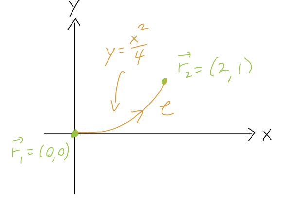
Consider the curve shown below. Which formula is the correct way to replace \( dx \) with \( dy \) in the line integral?
A. \( dx = \sqrt{2y}\ dy \)
B. \( dx = y\ dy \)
C. \( dx = \frac{2}{\sqrt{y}} dy \)
D. \( dx = \frac{1}{\sqrt{y}} dy \)
E. \( dx = \sqrt{\frac{2}{y}} dy \)
Answer: D
We can start by taking a differential of both sides of the curve equation \( y = x^2 / 4 \):
\[ \begin{aligned} dy = \frac{1}{4}(2x)dx = \frac{x}{2} dx \end{aligned} \]
or inverting,
\[ \begin{aligned} dx = \frac{2}{x} dy \end{aligned} \]
This option isn't listed to avoid confusion; although it is technically correct, it's not useful, because if we want to replace \( dx \) with \( dy \), we also need to replace \( x \) with \( y \) to do the integral. For that, we substitute in: \( y = x^2 / 4 \) means that \( x = \sqrt{4y} = 2\sqrt{y} \), leading to
\[ \begin{aligned} dx = \frac{1}{\sqrt{y}} dy \end{aligned} \]
No matter how we parameterize the curve, the result will always be the same - we're not changing anything except how we choose to describe it. Finding a good parameterization can be kind of an art (like choosing a good set of coordinates!) But the good news is that in physics applications, the parameterization is usually done for us: whenever we solve for the motion \( \vec{r}(t) \), the time \( t \) is already a parameter that describes the whole path.
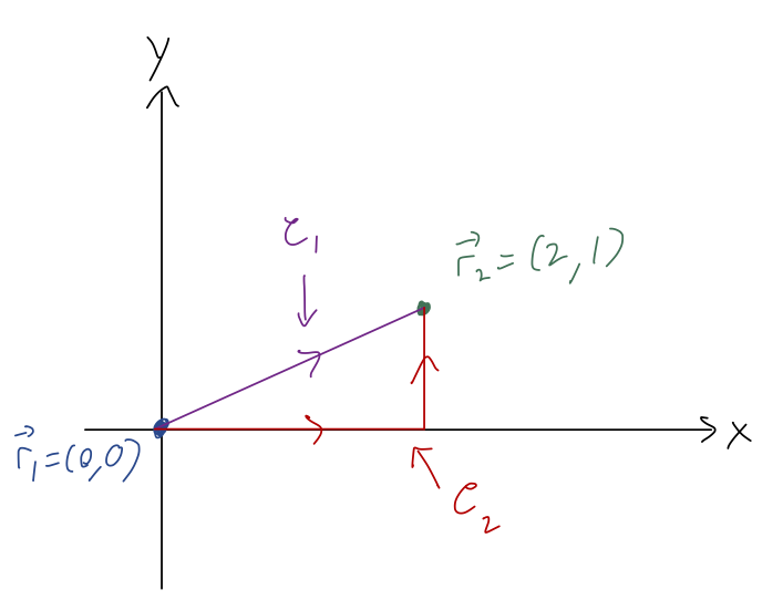
What can change the result of our curve, however, is taking a different path! Here's a simple example: consider the force
\[ \begin{aligned} \vec{F} = Fy\hat{x} \end{aligned} \]
Let's try with the same endpoints as before, now with the two paths shown in this figure:
Along \( \mathcal{C}_1 \), we already know that we can parametrize with e.g. \( dx = 2 dy \). In this case the force only has one component, so we see that
\[ \begin{aligned} W_1 = \int_{\mathcal{C}_1} \vec{F} \cdot d\vec{r} \\ = \int_{\mathcal{C}_1} (Fy dx) \\ = \int_0^1 Fy (2 dy) \\ = 2F \left.\frac{y^2}{2} \right|_0^1 = F. \end{aligned} \]
Now let's try the second path. This path isn't a smooth curve - it has a sharp corner where the path suddenly changes. This means that we should do the integral piecewise, meaning that we divide up the path into smooth parts and deal with them one at a time. Here, the pieces of the path are very simple: from the origin, we have the curve \( y = 0 \) (which also implies \( dy = 0 \)). For the second path of the curve, we have the fixed value \( x=2 \) - since this is constant, we see also that \( dx = 0 \). Thus, we can write the work integral along \( \mathcal{C}_2 \) as
\[ \begin{aligned} W_2 = \int_{\mathcal{C}_2} (Fy dx) \\ = F \int_0^2 (0) dx + F \int_0^1 y (0) = 0. \end{aligned} \]
So the work along the second path is different, it's just zero! (This is easy to see without doing the integrals, in fact; along the bottom edge the force \( \vec{F} \) is zero, and along the vertical edge we have \( \vec{F} \) perpendicular to \( d\vec{r} \).) This is an important point about work integrals, and line integrals in general: the result of a line integral can depend on the path.
Why did I write just "can depend" and not "always depends" on the path? Well, let's go back to our original force example \( \vec{F} = Fx \hat{x} + 2F \hat{y} \), and try that along the curve \( \mathcal{C}_2 \). As above, we split the line integral into two simple integrals:
\[ \begin{aligned} W_2 = \int_{\mathcal{C}_2} (F x dx + 2F dy) \\ = \int_0^2 F x dx + \int_0^1 2F dy \\ = 2F + 2F = 4F. \end{aligned} \]
In this particular case, we got the same answer again! In fact, this is not just a coincidence: you will get \( 4F \) for any path and this particular force. There is a deeper reason for this that we will see soon!
By the way, it's often useful to visualize what's going on in these line integrals before we just do the math out. Sketching the paths is only half of the visualization, because the direction and size of the force also matters. However, while the path is just a single line through space, the force \( \vec{F} \) is generally defined everywhere in space. As a result, we visualize it by drawing a force field plot. (A vector field is just a set of vectors that exist everywhere in space, whose values and directions are functions of position.)
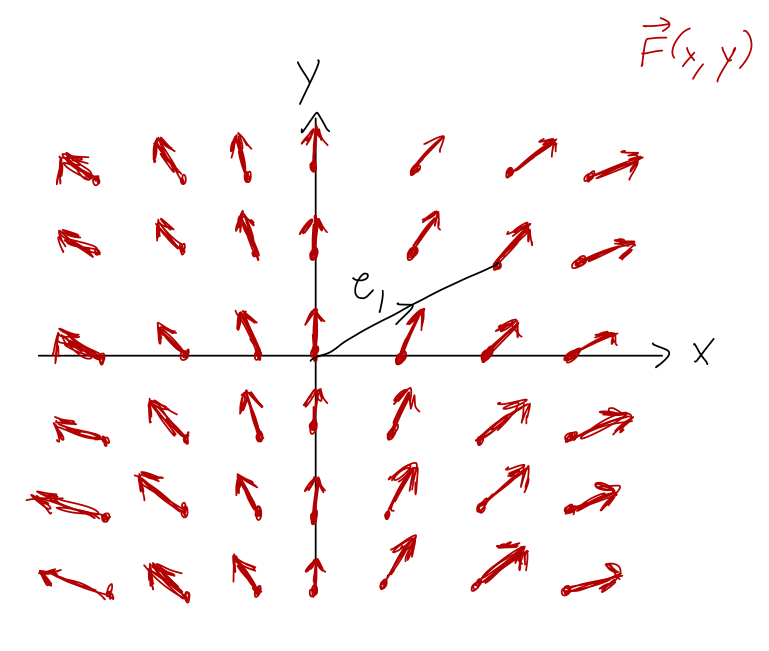
This makes it simpler to understand the work resulting from certain paths. (In particular, if we move perpendicular to the force field, then \( \vec{F} \cdot d\vec{r} \) is always zero and the work will be zero. More on that later...)
Since it's often useful to sketch vector fields, it's worth knowing that Mathematica has a function to do it for us, the VectorPlot[] function. Here's an example:
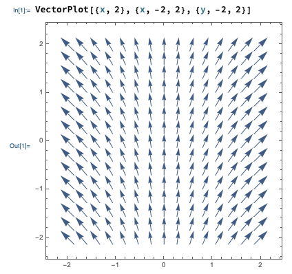
In Mathematica, vectors are denoted using curly braces {,}. You can see the input notation for VectorPlot above: the first argument is the vector field as a function, i.e. we enter {F_x, F_y} = {x, 2} for the vector field we've been working with. The last two arguments define the variable names and range to plot over, first x and then y.
Clicker Question
Which plot shows the force field for \( \vec{F} = -x \hat{x} - y \hat{y} \)?
A. 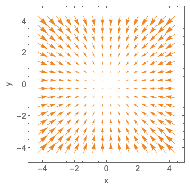
B. 
C. 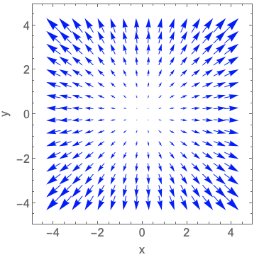
D. 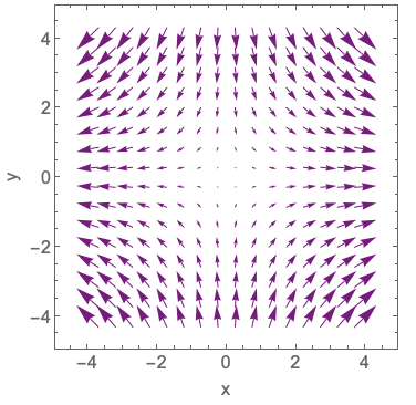
Answer: A
To answer this, we have to think about direction as well as magnitude. The \( -x \hat{x} \) component means that the vectors should be pointing towards the origin in the \( x \)-direction, and should get larger as we move further from the origin. We should see precisely the same in the \( \hat{y} \) direction for \( -y \hat{y} \). The only plots that look the same in the x and y directions are A and C; based on the sign, it has to be A. Alternatively, we can just use the criterion that both components have to always point towards the origin, which is violated by every plot except A.
Another way to solve this is to realize that \( -x \hat{x} - y \hat{y} = -\vec{r} \), i.e. the force is proportional to (minus) the position vector, which again leads us to option A.
This is a very important example of a force, by the way - this is in fact a plot of the spring force \( \vec{F}_k = -k\vec{r} \) in two dimensions! Try to visualize it for a point mass connected to the origin by a spring.