We started with a line integral example which I posted in the last set of lecture notes, then we went back to conservative forces, which as a reminder must satisfy the following two conditions:
- Conservative forces depend only on \( \vec{r} \) and constants.
- The work done by a conservative force from \( \vec{r}_1 \) to \( \vec{r}_2 \) is independent of the path taken.
Clicker Question
Which of the following forces are not conservative (violating either condition 1 or condition 2?)
- Gravity near the Earth's surface
- Air resistance
- Friction
- Electric force, with a time-dependent source
A. Only 2 is not conservative.
B. 2 and 3 are not conservative.
C. 2, 3, 4 are not conservative.
D. 1, 2, 3 are not conservative.
E. None of them are conservative.
Answer: C
Let's start with the most obvious cases: air resistance is not conservative since it depends on \( \vec{v} \), which directly violates condition 1 (that it should only depend on \( \vec{r} \).) The electric force is normally conservative, but if the electric field is time-dependent, then condition 1 is violated again: if it depends on time, it doesn't just depend on \( \vec{r} \).
Next, we come to friction. Friction is a tricky example: in terms of condition 1, it depends a little bit on \( \vec{v} \) - whether \( \vec{v} = 0 \) determines static vs. kinetic friction, and the direction of friction depends on the direction of \( \vec{v} \). If we just restrict to motion in a constant direction, then friction can (temporarily) look okay under condition 1. However, it will always violate condition 2, even in this case. If the frictional force is constant, then its work done will be \( |\vec{F}| L \) over a path of length \( L \) - which means it matters which path we take!
Finally, gravity. If we're near the Earth's surface, gravity is just a constant vector (approximately), so it doesn't depend on any other variables and condition 1 is good. (The general form of the gravitational law is \( F_g = GmM / r^2 \), which indeed only depends on \( \vec{r} \), so condition 1 is okay everywhere.) Condition 2, path independence, is guaranteed by the existence of the gravitational potential as we just discussed. Near the Earth's surface, this is the familiar \( mgh \); even in the general case, there is a gravitational potential function as we'll see in more detail soon. Gravity is always conservative.
Back to our general discussion of potential energy \( U \). Assuming for the moment that the corresponding \( \vec{F} \) is the only force acting, the work-KE theorem applies:
\[ \begin{aligned} T(\vec{r}_2) - T(\vec{r}_1) = W_{1 \rightarrow 2} = \int_{\vec{r}_1}^{\vec{r}_2} \vec{F} \cdot d\vec{r} = -U(\vec{r}_2) + U(\vec{r}_1) \end{aligned} \]
or rearranging,
\[ \begin{aligned} T(\vec{r}_1) + U(\vec{r}_1) = T(\vec{r}_2) + U(\vec{r}_2). \end{aligned} \]
In other words, the combination
\[ \begin{aligned} E = T + U, \end{aligned} \]
which we call the mechanical energy (or just "the energy" when we're doing classical mechanics), doesn't change as we move from \( \vec{r}_1 \) to \( \vec{r}_2 \). Since this is true for any two points we choose, and since the path and other variables can't change the work, we see that in the presence of a conservative force, energy is conserved:
\[ \begin{aligned} \frac{dE}{dt} = 0. \end{aligned} \]
Since we used the work-KE theorem, we technically assumed above that \( \vec{F} \) is the only force acting in our system. If we have multiple forces, remember that we can divide net work up into the sum of work due to each individual forces. If they're all conservative, then we can write a separate potential energy function for each force. So the more general version of the mechanical energy is
\[ \begin{aligned} E = T + U_1 + U_2 + U_3 + ... \end{aligned} \]
if we have several forces \( \vec{F}_1, \vec{F}_2, \vec{F}_3... \)
Of course, as we just noted there are plenty of non-conservative forces around. The work-KE theorem still applies to them, and we can still split them up. If we have both conservative and non-conservative forces, then
\[ \begin{aligned} \Delta T = W_{\rm net} = W_{\rm cons} + W_{\rm non-cons} \\ = -\Delta U + W_{\rm non-cons} \end{aligned} \]
or
\[ \begin{aligned} \Delta E = W_{\rm non-cons} \end{aligned} \]
So energy is not conserved if we have non-conservative forces, but we know exactly how it will change if we keep track of the work done by those forces.
Here's a quick note about the deeper interpretation of this absence of energy conservation, since I commented early that conservation of energy is a really important and general physical principle. Friction and air resistance are not fundamental forces: ultimately, they come from electromagnetic forces between the atoms in our object and the surface or medium providing the force. All of the known fundamental forces of nature are conservative, which means that total energy is conserved, period. When we find a non-zero \( \Delta E \) due to something like friction, that "lost" energy is just being transferred into another form - mostly heat, in the case of friction. When multiple conservative forces are present, energy will be exchanged between the different potentials and kinetic energy (see here for a classic example!), but total \( E \) is always the same.
One more brief aside, about magnetic fields, which are sort of a weird example. They are non-conservative because they depend on speed, but they also don't do any work at all because the magnetic force is always perpendicular to \( \vec{v} \)! So a system including a magnetic field will still conserve mechanical energy - but we can't write a potential energy function to describe the motion. (In other words, conserving energy alone isn't sufficient for a force to be "conservative" by the definition we're using.) Normal forces are even weirder, but they fall into the same category as magnetic force: they usually don't do any work at all, but they're not technically considered to be conservative and we can't use potential energy to describe normal forces.
At this point, Taylor does an example of mixing conservative and non-conservative forces, involving a sliding block with friction. We solved the sliding block with friction way back in chapter 1, but work gives a quicker way to find the speed as a function of the height of the block. I'll skip this example because Taylor already did it, and unfortunately there aren't any other good simple examples of this sort of thing: you could try to do a similar trick with linear air resistance, but the equations are unsolvable and you have to resort to numerics anyway, so using energy and work doesn't really help.
Example: potential in an electric field
Let's do a concrete example: a charge \( +q \) is suspended in a uniform electric field, \( \vec{E} = E_0 \hat{x} \). The force on the charge is proportional to the field
\[ \begin{aligned} \vec{F} = q\vec{E} = qE_0 \hat{x}. \end{aligned} \]
The force due to a (static) electric field is conservative, so we can go ahead and calculate a potential energy function by using the definition:
\[ \begin{aligned} U(\vec{r}) = -\int_{\vec{r}_0}^{\vec{r}} \vec{F} \cdot d\vec{r} = -\int_{\vec{r}_0}^{\vec{r}} qE_0 dx. \end{aligned} \]
Normally, to continue we'd need to pick a reference point \( \vec{r}_0 \) and a path to integrate along - even if we know the answer will be path-independent, we have to choose one! However, in this case since the force is constant, we can see that the path doesn't matter at all: the result of the integral is
\[ \begin{aligned} U(\vec{r}) = -qE_0 (x - x_0) \end{aligned} \]
or simply \( U(x) = -qE_0 x \) if we pick \( \vec{r}_0 \) to be the origin \( (0,0,0) \), which is clearly the simplest choice. This is a rare example where we can immediately tell that a force is conservative just by trying to calculate the work.
Let's think briefly about the answer: we see that since \( U(x) \sim -x \), the potential decreases as \( x \) increases. This makes sense, since the electric field will push our charge in the \( +\hat{x} \) direction; as it moves it will pick up kinetic energy \( (\Delta T > 0) \), so energy conservation requires that it lose an equal amount of potential energy \( (\Delta U < 0.) \) This should remind you of what you already know about gravitational potential \( U(z) = +mgz \) near the Earth's surface.
Example: another conservative force
Let's go back to the example force that we were looking at to start our discussion of line integrals,
\[ \begin{aligned} \vec{F} = Fx\hat{x} + 2F\hat{y}. \end{aligned} \]
I mentioned in passing that it wasn't a coincidence that we kept finding the same answer for different paths with this force - it is, in fact, conservative. So let's find the potential energy function:
\[ \begin{aligned} U(\vec{r}) = -\int_{\vec{r}_0}^{\vec{r}} \vec{F} \cdot d\vec{r} = -\int_{\vec{r}_0}^{\vec{r}} Fx' dx' + 2F dy'. \end{aligned} \]
(I'm using primed coordinates under the integral to avoid some confusion.) For simplicity, let's take \( \vec{r}_0 \) to be the origin again. In order to do this integral and find \( U(\vec{r}) \), this time we will need to pick a path. Vector field plots are always a useful place to start when deciding on a path! Here's the field plot for this force field once again:
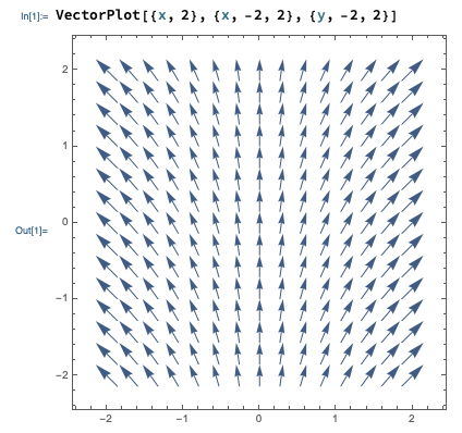
This is a little abstract, since our path has to be valid for any choice of \( x \) and \( y \), but any sufficiently general curve will do. For example, we can take a straight-line path, but if we do that we have to let the slope be variable. Letting \( y' = bx' \), we have \( dy' = b dx' \), which we can use to simplify down the integral:
\[ \begin{aligned} U(\vec{r}) = -\int_0^{x} Fx' dx + 2F (b dx') \\ = -\frac{1}{2} F x^2 - 2Fbx. \end{aligned} \]
Now we have to deal with the slope \( b \) - we introduced that variable with our path choice, so we have to get rid of it. Remember that we're finding the potential at a given point \( \vec{r} = (x,y,z) \). For the path to reach that point, we must also have \( y = bx \), or \( b = y/x \). Plugging back in gives us our answer:
\[ \begin{aligned} U(x,y) = -\frac{F}{2} (x^2 + 4y). \end{aligned} \]
Just to make sure, let's re-compute the answer using another path. In fact, although the straight-line path was simple to set up, it's not really the simplest path we can use. Generally, moving along or perpendicular to field lines whenever possible will simplify our line integrals. Let's do a piecewise path where we move along the \( y \)-axis first (so \( dx = 0 \)), and then horizontally in the \( x \) direction (so \( dy = 0 \)). This splits our answer into two integrals:
\[ \begin{aligned} U(\vec{r}) = -\int_0^y 2F dy' - \int_0^x Fx' dx' \\ = -2Fy - \frac{1}{2} F x^2 \end{aligned} \]
exactly as we found with the straight-line path, but now in just one step!
Force from the potential
Let's come back to the relationship between potential energy and force. We defined the potential based on a path integral of the force:
\[ \begin{aligned} U(\vec{r}) = -\int_{\vec{r}_0}^{\vec{r}} \vec{F} \cdot d\vec{r}, \end{aligned} \]
which uses \( \vec{F} \) to find \( U \). But we know that regular integrals can be inverted using derivatives, so it's natural to ask: can we go the other way here as well, i.e. can we find \( \vec{F}(\vec{r}) \) given \( U(\vec{r}) \)?
The answer is yes, and the easiest way to see it is thinking about the infinitesmal version of the integral above. Remember that a line integral is just a sum over lots of infinitesmal segments, which means that we can go backwards and notice that an infinitesmal contribution to the potential energy takes the form
\[ \begin{aligned} dU = -\vec{F} \cdot d\vec{r} \end{aligned} \]
(you can think of this as the change in potential if we move \( \vec{r} \) by a tiny amount; also, we get the formula above back by integrating both sides.) There's another way to write out \( dU(\vec{r}) \); by using the chain rule with respect to the individual coordinates, we have
\[ \begin{aligned} dU = \frac{\partial U}{\partial x} dx + \frac{\partial U}{\partial y} dy + \frac{\partial U}{\partial z} dz. \end{aligned} \]
We can write out the first version of \( dU \) in a very similar way by expanding the dot product:
\[ \begin{aligned} dU = -F_x dx - F_y dy - F_z dz \end{aligned} \]
These equations are both \( dU \), so their right-hand sides have to be equal. But more than that, they have to be equal for any possible path that we choose! Changing a path will change how \( dx \), \( dy \), and \( dz \) vary, which means that for these equations to always be true, the things multiplying \( dx \), \( dy \), and \( dz \) must be equal. This gives us the result
\[ \begin{aligned} \vec{F} = -\frac{\partial U}{\partial x} \hat{x} - \frac{\partial U}{\partial y} \hat{y} - \frac{\partial U}{\partial z} \hat{z} \end{aligned} \]
or written more compactly,
\[ \begin{aligned} \vec{F} = -\vec{\nabla} U \end{aligned} \]
where \( \vec{\nabla} \) represents the gradient of the function \( U \). (The upside-down triangle symbol is usually called 'del', although another common name is 'nabla', which comes from the Greek word for 'harp'.) The gradient can be thought of as being defined through the equation
\[ \begin{aligned} \vec{\nabla} \equiv \frac{\partial}{\partial x} \hat{x} + \frac{\partial}{\partial y} \hat{y} + \frac{\partial}{\partial z} \hat{z} \end{aligned} \]
in Cartesian coordinates. Clearly from the way we found it, \( \vec{\nabla} \) acts as the inverse operation to a regular line integral, just as an ordinary derivative is the inverse of an ordinary integral. (Because it is a vector, \( \vec{\nabla} \) will look different if we change coordinates! I won't go through those formulas for now, just warn you that it will happen.)
If you have more of a formal math background, you might recognize \( \vec{\nabla} \) as a sort of object called an operator. An operator is basically a map from one class of objects to another. In this case, it takes us from a scalar function \( U(x,y,z) \) to a vector function \( \vec{F}(x,y,z) \). You probably remember the two other common vector differential operators: the divergence \( (\vec{\nabla} \cdot) \), which takes a vector to a scalar, and the curl \( (\vec{\nabla} \times) \), which takes a vector to another vector. We'll see more of them soon! If you've seen something like \( d/dx \) written on its own, that's also an example of an operator.