In one dimension, equipotential surfaces aren't useful anymore - they would consist of some scattered points. Instead, we can visualize a problem by just plotting \( U(x) \) vs. \( x \). For example, here is the potential \( U(x) = \frac{1}{2} kx^2 \) corresponding to a mass on a spring, which is unstretched at \( x=0 \):
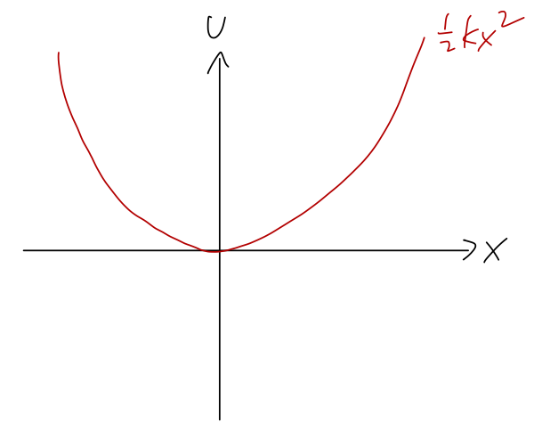
Again, the direction of the force is always "downhill", opposite the direction of increasing \( U \). We can also clearly see that there is an equilibrium point at \( x=0 \), where the potential is flat (\( dU/dx=0 \)) and therefore the force vanishes. (Equilibrium just means that the system will stay there if we start it there at rest.)
The potential carries a lot of useful information about a physical system, even in cases where we can't solve it completely! Once again, gravity will be a useful example and metaphor for understanding potentials in general. Imagine a roller coaster on a track. As a function of the distance \( x \) along the track, the height of the track \( y(x) \) will vary, usually in some complicated and interesting way. Since the gravitational potential is \( U(y) = +mgy \), that means that drawing the track is the same thing as drawing the potential energy!
Suppose we have a segment of roller coaster track that looks like this:
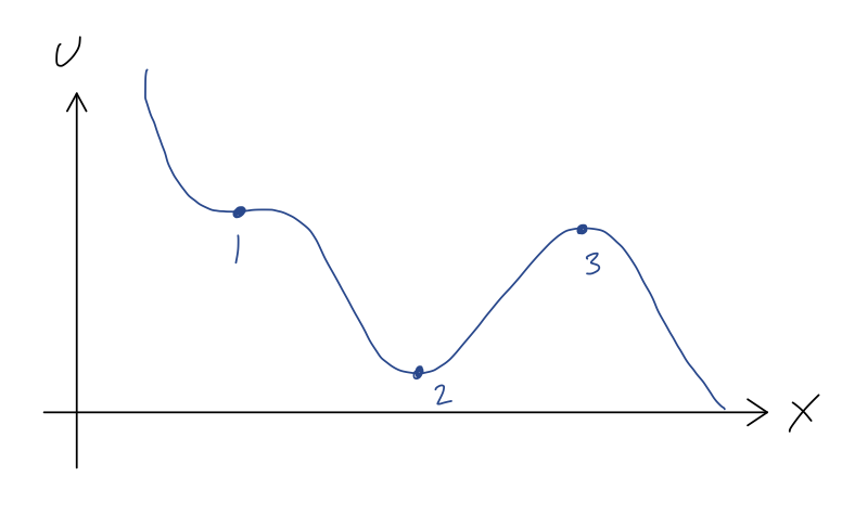
We can immediately see the points of equilibrium, marked 1, 2, and 3, where the force will vanish, and thus where the roller coaster cart would remain if it started at rest. We also get an immediate sense for the stability of these equilibria. A stable equilibrium point is one for which the system will remain near the equilibrium point if pushed slightly away; we can see that this is true at point 2, since if we give the cart a small push from this point, the force will always be directed back towards the lowest point.
An unstable equilibrium point is the opposite, a point where a small push will result in a large change in the system's position. This is clearly the case at point 3; for a small push away from point 3, the force points away from point 3, and the coaster will accelerate away - back towards point 2, or off to the right, depending on which way we push it.
We can be more rigorous about these statements by considering a Taylor series expansion around each of these points. Let's start with point 2, and I'll use the shorthand notation \( U'(x) = dU/dx \) here. Since we already know that \( U'(x_2) = 0 \), the series expansion looks like
\[ \begin{aligned} U(x) \approx U(x_2) + \frac{1}{2} U''(x_2) (x-x_2)^2 + ... \end{aligned} \]
Now, we can't actually compute the second derivative, but we do know from the plot that it must be positive. (Our series expansion is telling us that \( U(x) \) looks like a parabola if we get close enough to \( x_2 \), and from the plot the parabola has to be opening upwards.) So if we define \( U''(x_2) = +k \) with \( k>0 \), then
\[ \begin{aligned} U(x) \approx U(x_2) + \frac{1}{2} k(x-x_2)^2 + ... \end{aligned} \]
near point 2. Taking the derivative of this series gives us the force,
\[ \begin{aligned} F(x) = -\frac{dU}{dx} = -k(x-x_2). \end{aligned} \]
This looks exactly like a spring force; it points towards \( x_2 \), no matter what value of \( x \) we use. We can go a step further and solve for the motion. Let's change coordinates so that \( u = x-x_2 \) is the distance to point 2. Then \( F(u) = -ku \), and the equation of motion is
\[ \begin{aligned} m\ddot{u} = -ku. \end{aligned} \]
We haven't considered general second-order ODEs yet, but we do know that this is a linear ODE, so it has a general solution containing 2 unknown constants, and we just need to find two different functions that go back to themselves with a minus sign after two derivatives. The basic trig functions both satisfy this property, so the solution is
\[ \begin{aligned} u(t) = A \cos (\sqrt{k/m} t) + B \sin (\sqrt{k/m} t). \end{aligned} \]
We don't need any more detail than this: the point is that since \( \sin \) and \( \cos \) both oscillate between \( -1 \) and \( +1 \), our total solution is bounded - it will always stay within some range of point 2.
If we expand around point 3, we find an almost identical story, except that now we find \( U''(x_3) = -\kappa \) with \( \kappa > 0 \), which gives us the equation of motion
\[ \begin{aligned} m\ddot{u} = +\kappa u \end{aligned} \]
now with \( u = x-x_3 \). Without the minus sign, the solutions we find are exponentials instead of trig functions:
\[ \begin{aligned} u(t) = Ae^{-\sqrt{\kappa/m} t} + Be^{+\sqrt{\kappa/m} t}. \end{aligned} \]
The second exponential term gets arbitrarily large as \( t \) gets bigger, so our solution is indeed unstable - it will run away from point \( x_3 \). Of course, the motion isn't exponential forever; we're doing a series expansion around \( x_3 \), so as soon as we get far enough away that the terms we dropped from the series become important, we can't use this simple solution for \( x(t) \) anymore.
Finally we come to point 1, which is sort of a tricky case; it is a saddle point of \( U(x) \), which means that the direction of the force depends on which way we push the cart. In physical terms, this is also an unstable equilibrium point. To see why, let's Taylor expand one more time. We still know that \( U'(x_1) = 0 \), but we must also have \( U''(x_1) = 0 \). (You may remember from calculus that this is the condition for a saddle point. More physically, if \( U''(x_1) \) wasn't zero, then close enough to \( x_1 \) our function would have to look parabolic, but that would mean it has to look like point 2 or point 3.) Thus, the series expansion here is
\[ \begin{aligned} U(x) \approx U(x_3) + \frac{1}{3!} U'''(x_3) (x-x_3)^3 + ... \end{aligned} \]
If we let \( U'''(x_3) = -q \) with \( q > 0 \) (convince yourself from the graph!), then the equation of motion is
\[ \begin{aligned} m\ddot{u} = \frac{1}{2} qu^2. \end{aligned} \]
We can't solve this analytically - there is no solution using elementary functions. But we don't need to, because it tells us what we need to know: the acceleration \( \ddot{u} \) is always positive, no matter the sign of \( u \) itself. So if we displace the cart from point 1 in either direction, it will be accelerated to the right - and since the acceleration increases as \( u \) increases, this solution is unstable and the cart moves away from point 1.
Equilibrium points are local statements about a physical system, but we can also say interesting and useful things about the global behavior using the one-dimensional potential. Let's think about how this works with some clicker questions!
Clicker Question
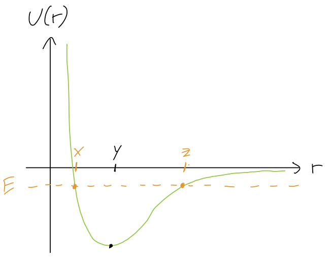
The plot below shows a sketch of the one-dimensional potential for a two-atom molecule, as a function of the inter-atomic distance \( r \). Suppose the total energy of this system \( E \) is negative, as shown in the sketch. What does the motion of the two atoms look like?
A. The distance is constant, \( r = y \).
B. The distance oscillates between \( r=x \) and \( r=z \).
C. The distance oscillates around \( y \), but doesn't reach \( r=x \) or \( r=z \).
D. The molecule is unbound (the atoms fly apart, \( r \rightarrow \infty \).)
Answer: B
The key here is that \( E = T + U \) is always conserved (this is why we can draw \( E \) as a straight line!) We thus have the usual trade-off, that \( T \) increases as \( U \) decreases and vice-versa. But unlike \( U \), the kinetic energy \( T \) has a very important property: it can never be negative! Another way to say this: whenever \( E = U \), we have \( T = 0 \), so our object comes to a stop. These points are known as turning points, because the object can't continue moving past them to negative \( T \) - it has to turn around.
We can read off the plot, then, that \( r = x \) and \( r = z \) are turning points, and the atomic distance is trapped between them - answer B.
Clicker Question
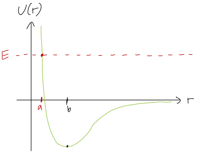
Continuing with the same molecule, now suppose the total energy \( E > 0 \). What does the motion look like?
A. The distance is constant, \( r=a \).
B. The distance oscillates back and forth around \( r=b \).
C. The molecule is unbound (the atoms fly apart, \( r \rightarrow \infty \).)
D. None of the above.
Answer: C
Exactly like the previous example, but now there's only a single turning point. As \( r \) gets larger and larger, \( T \) remains non-zero with \( E > 0 \), so we see that the atoms can just keep moving apart forever, giving us answer C.
You might ask what happens if the initial condition is that \( r \) is decreasing. This will mean that \( r \) approaches the turning point at \( r = a \), at which point the motion will reverse. We can't tell which way the motion is at a given time based on the energy, since \( T = \frac{1}{2} mv^2 \) is the same whether \( v \) is positive or negative. But we know that if we wait long enough, the long-term motion will still be \( r \) increasing towards infinity.
Clicker Question
Finally, for the same molecule, which is the correct sketch of the kinetic energy \( T(x) \)? (This is for the most recent case where \( E > 0 \).)
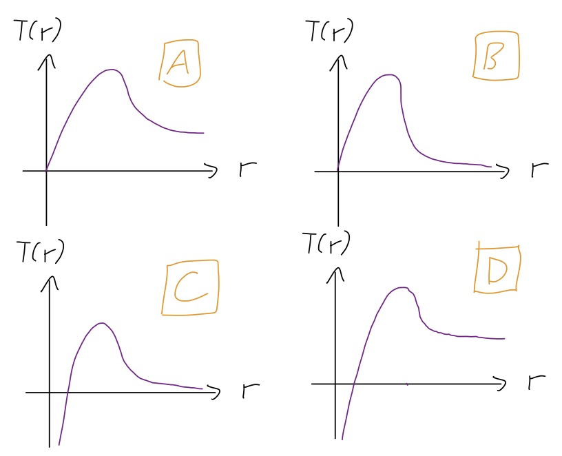
Answer: D
We used kinetic energy in the previous two answers, but spotting where \( T = 0 \) is a little easier than visualizing the whole curve! Still, this is just a simple use of the relationship \( E = T - U \), so we basically flip the curve upside-down.
(Note: in class, I showed a bad version of this where option D was different and all of the options were wrong! Full credit for any answers on this one, due to my mistake.)
Let's recap: since total energy \( E = T + U \) is conserved, if we know \( U(x) \) and the total energy, then we also know \( T(x) \). Instead of making a new plot, it's often useful to just draw the value of \( E \) as a dotted line on the plot for \( U(x) \).
For example, let's go back to our roller coaster and suppose the system begins at rest halfway between points 1 and 2. Then \( E = U(x_0) \), since at rest \( T=0 \). Let's draw it on the graph:
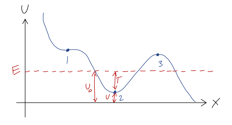
Since \( E = T + U \) and \( E \) is always the same, the difference between our dashed \( E \) line and the \( U(x) \) curve at any point is exactly the kinetic energy \( T \)! Now, since \( T = mv^2/2 \), it has the very important property that it can never be negative (note that \( U \) can be negative, and so can \( E \), because the value \( U=0 \) is arbitrary.) But that means that we can never have \( U > E \). So for the value of \( E \) shown, the cart can never reach point 1, point 3, or any part of the track above \( E \)!
This is a very simple but powerful observation: without knowing any of the details about how the cart moves with time, we know that its motion will never take it beyond the values of \( x \) where \( E = U(x) \) (the turning points.) The regions of the track where \( U > E \) are known as forbidden regions; we know the cart can never be found there. If all we know is \( E \), then the cart could be anywhere else; in this example, it could be in the potential well near point 2, or it could be on the downward-sloping track to the right of point 3. If we also know where the cart starts, then we can identify it as being stuck in one of these two regions, and it can never get to the other one. (Of course, as you know from modern physics, this is only true classically; a quantum roller coaster would be able to tunnel from one region to the other.)
Example: the pendulum, revisited
We've previously talked about the motion of a simple pendulum, and found the equation of motion awhile ago to be
\[ \begin{aligned} \ddot{\phi} = -\frac{g}{L} \sin \phi \end{aligned} \]
This is a non-linear differential equation, and there is no simple analytic solution to it at all. The usual procedure is to use the small-angle approximation, or numerical solution. But since this is a one-dimensional problem, we can instead write down the potential energy to make some useful observations!
Once again, here's a sketch of the pendulum setup:
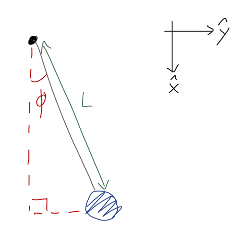
The only force acting is gravity, in the \( \hat{x} \) direction as the coordinates are drawn. Let's set the gravitational potential to be zero at the lowest point of the pendulum, when \( \phi = 0 \). With the origin at the pendulum support, we thus have
\[ \begin{aligned} U(x,y) = mg(L-x) = mgL(1 - \cos \phi) \end{aligned} \]
using \( x = L \cos \phi \). It's always a good idea to check that the sign makes sense here, so let's think about it: at \( \phi = 0 \), we have \( U = 0 \) as desired. At \( \phi = \pi/2 \), we have \( U = mgL \); the gravitational potential should be larger when the bob is higher, so this also checks out.
Let's sketch the potential as \( \phi \) changes from 0 to \( 2\pi \):
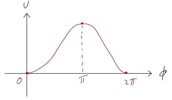
So we see two equilibrium points: in addition to the expected \( \phi = 0 \), there is also an unstable equilibrium at \( \phi = \pi \). This might seem a little weird, but if you think about it for a moment it makes intuitive sense: at exactly \( \phi = \pi \) the pendulum is perfectly balanced straight above the support.