Last time, we set up the example of a simple pendulum:
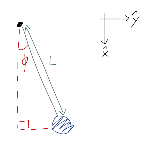
with potential energy function
\[ \begin{aligned} U(\phi) = mgL(1 - \cos \phi). \end{aligned} \]
We talked about using a graph of the potential to obtain the equilibrium points; now let's exercise our Taylor series abilities to check the stability or instability of the two equilibrium points algebraically. To find equilibrium points in general, we solve for where the gradient of \( U \) vanishes, or:
\[ \begin{aligned} \frac{dU}{d\phi} = 0 = mgL \sin \phi \end{aligned} \]
which has solutions at \( \phi = 0, \pi, 2\pi, ... \), matching the points I already marked on the graph. Next, if we series expand the potential first at \( \phi = 0 \), we have
\[ \begin{aligned} U(\phi) \approx U(0) + \frac{1}{2} U''(0) \phi^2 + ... \\ = mgL(1 - \cos 0) + \frac{1}{2} (mgL \cos 0) \phi^2 + ... \\ = \frac{1}{2} mgL \phi^2 + ... \end{aligned} \]
which is indeed a stable equilibrium, since the coefficient of \( \phi^2 \) is positive. Note that I skipped the \( U' \) term in the expansion, since I already know it's zero at this point. Let's repeat the exercise at \( \phi = \pi \),
\[ \begin{aligned} U(\phi) \approx U(\pi) + \frac{1}{2} U''(\pi) (\phi-\pi)^2 + ... \\ = mgL(1 - \cos \pi) + \frac{1}{2} (mgL \cos \pi) (\phi-\pi)^2 + ... \\ = 2mgL - \frac{1}{2} mgL (\phi-\pi)^2 + ... \end{aligned} \]
which is indeed unstable: the potential looks like a downwards parabola near the point, and if we compute the force
\[ \begin{aligned} F(\phi) = -\frac{dU}{d\phi} = mgL(\phi - \pi) \end{aligned} \]
it will always point in the same direction as \( \phi \) if we move slightly away from the equilibrium, and we will be pushed away.
Moving beyond equilibrium, we can also use conservation of energy and turning points to say useful things about the motion, without having to assume a small angle. Suppose the pendulum starts at \( \phi = 0 \), and we give it a push so that it starts moving with initial speed \( v_0 \). What does its motion look like? The total energy is just \( T \) at \( \phi = 0 \), so we have
\[ \begin{aligned} E = T + U \\ \frac{1}{2} mv_0^2 = T + mgL(1 - \cos \phi) \end{aligned} \]
The turning points \( \phi_T \) occur where \( T = 0 \), or
\[ \begin{aligned} \frac{1}{2} mv_0^2 = mgL (1 - \cos \phi_T) \\ 1 - \cos \phi_T = \frac{v_0^2}{2gL} \\ \Rightarrow \cos \phi_T = \left( 1 - \frac{v_0^2}{2gL} \right). \end{aligned} \]
So although we don't know the detailed motion as a function of time, it's easy to find the maximum possible angle the pendulum will reach based on the initial speed. Notice that this works for any angle, but only for \( v_0^2 < 4gL \), at which point \( \phi_T = \pi \). For even larger initial speeds, there is no solution: we just have \( E > U \) everywhere, and the pendulum will just spin in a circle forever, in the absence of other forces.
If we really want to know about the motion as a function of time, there's one more nice trick we can do in one dimension. For any potential at all, the relation \( E = T + U \) in one dimension can be rewritten as:
\[ \begin{aligned} \frac{1}{2} m \dot{x}^2 = E - U(x). \end{aligned} \]
which we can solve for \( \dot{x} \):
\[ \begin{aligned} \dot{x} = \pm \sqrt{\frac{2}{m}} \sqrt{E - U(x)} \end{aligned} \]
(we would need extra information to figure out the sign, since \( T \) is the same for \( +\dot{x} \) and \( -\dot{x} \).) This is a first order and separable ODE - no matter how complicated \( U(x) \) is! So we can use it to write down a completely general solution: if \( x(0) = x_0 \), then
\[ \begin{aligned} t(x) = \pm \sqrt{\frac{m}{2}} \int_{x_0}^x \frac{dx'}{\sqrt{E-U(x')}} \end{aligned} \]
which we then have to invert to get \( x(t) \).
For the pendulum, this becomes
\[ \begin{aligned} t(\phi) = \pm \sqrt{\frac{m}{2}} \int_{\phi_0}^\phi \frac{d\phi'}{\sqrt{E - mgL(1 - \cos \phi')}} \end{aligned} \]
This is, unfortunately, one of those integrals that you can't actually do: it is used to define a special function called an elliptic function, which is the solution to the pendulum at all angles. So we didn't get something for nothing in this case. On the other hand, this can be a convenient way to do a numerical solution, since you don't need an ODE solver like Mathematica - you just need to do an integral.
Taylor explores a few other special topics in energy conservation, including the use of time-dependent potential energies (Taylor 4.5) and some more explorations of equilibrium and one-dimensional systems (4.7); I encourage you to read about these for your interest, but we won't go into them in any detail. Instead, we'll continue with his discussion of central forces, which will lead us into a detailed case study of the most important fundamental force in mechanics: gravity.
Central forces
A central force is one for which in some choice of coordinates,
\[ \begin{aligned} \vec{F}(\vec{r}) = f(\vec{r}) \hat{r}. \end{aligned} \]
The concept is that the origin (i.e. the center of our coordinate system) is the source providing our central force, and the force at any point \( \vec{r} \) always points towards or away from this center. This should remind you a bit of drag forces, which we argued were always in the direction of \( \hat{v} \) (or opposite \( \hat{v} \), more precisely.) In both cases, we have a specific direction for the force by identifying where it comes from (motion for air resistance, and the source object for central force.)
Clicker Question
Which is the correct form of the gravitational force on mass 2, due to mass 1 (at the origin)?
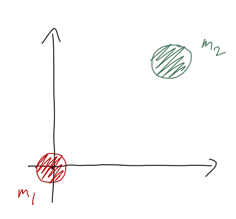
A. \( \vec{F}_g = +\frac{Gm_1 m_2}{r^2} \hat{r} \)
B. \( \vec{F}_g = -\frac{Gm_1 m_2}{r^2} \hat{r} \)
C. \( \vec{F}_g = +\frac{Gm_1 m_2}{r^3} \vec{r} \)
D. \( \vec{F}_g = -\frac{Gm_1 m_2}{r^3} \vec{r} \)
E. More than one of the above is correct.
Answer: E
This is a warm-up to get us thinking about magnitude and direction for central forces. We know that the gravitational force is always attractive, so since we're asking about the force on mass 2, it should point in the \( -\hat{r} \) direction, towards mass 1 at the origin. This means either B or D is correct. But B and D are actually the same formula! If we plug in the definition \( \vec{r} = r \hat{r} \) to D, we get B. So the answer is E - both options are correct!
You might wonder why we would ever write this in form D, instead of form B. We'll see this in detail soon, but the short answer is that gravity problems will involve integration over \( \vec{F}_g \), and \( \vec{r} = x \hat{x} + y \hat{y} + z \hat{z} \) is simple to write out in components - whereas \( \hat{r} \) has the extra factor of \( 1/r = 1/\sqrt{x^2 + y^2 + z^2} \) to deal with.
We'll deal with gravity in great detail soon. Another good example that you already know of a central force is just the electric force: if I put a charge \( Q \) at the origin, then the force on a second charge \( q \) sitting at point \( \vec{r} \) is
\[ \begin{aligned} \vec{F}_e(\vec{r}) = \frac{kqQ}{r^2} \hat{r}. \end{aligned} \]
As Taylor observes, this (along with gravity, which has the same \( r \) dependence) is a slightly more specialized version of a central force, because \( f(\vec{r}) = f(r) \), i.e. the magnitude of the force only depends on the distance between the charges. This is an example of spherical symmetry, or rotational invariance: in spherical coordinates, we can rotate our test charge \( q \) around in \( \theta \) and \( \phi \) as much as we want, and as long as \( r \) is held fixed the force magnitude is the same (although the direction changes so it's always pointing out from the origin.) As we'll prove in a moment, this is related to the question of whether or not we have a conservative central force. A static electric force is definitely conservative!
Gradient and curl in spherical coordinates
To study central forces, it will be easiest to set things up in spherical coordinates, which means we need to see how the curl and gradient change from Cartesian. Let's go through the derivation for the gradient - although this is something you can always look up, it's actually pretty easy, and the formula that you look up won't seem so arbitrary. Remember that in our derivation of gradient, we found the following infinitesmal relationship:
\[ \begin{aligned} dU = \vec{\nabla} U \cdot d\vec{r}. \end{aligned} \]
We have previously looked at how \( d\vec{r} \) changes if we switch coordinates: we can always start with the Cartesian version
\[ \begin{aligned} d\vec{r} = dx \hat{x} + dy \hat{y} + dz \hat{z} \end{aligned} \]
and just substitute in the change from \( (x,y,z) \) to \( (r,\theta,\phi) \). However, in this case it's probably easier to just start in spherical coordinates, where we know that simply \( \vec{r} = r \hat{r} \), and so taking the derivative with respect to some parameter \( s \),
\[ \begin{aligned} \frac{d\vec{r}}{ds} = \frac{dr}{ds} \hat{r} + r \frac{d\hat{r}}{ds}. \end{aligned} \]
Now we can relate the unit vector back to Cartesian coordinates:
\[ \begin{aligned} \hat{r} = \frac{1}{r} \left( x \hat{x} + y \hat{y} + z \hat{z} \right) \\ = \sin \theta \cos \phi \hat{x} + \sin \theta \sin \phi \hat{y} + \cos \theta \hat{z}. \end{aligned} \]
We can take a derivative with respect to \( s \) here, but it's better to remember that we eventually want our answer in terms of spherical unit vectors. Remember that we define the unit vectors as pointing in the direction of change with respect to a certain coordinate, so we can find them by looking at the derivatives of \( \hat{r} \):
\[ \begin{aligned} \frac{d\hat{r}}{d\theta} = \cos \theta \cos \phi \hat{x} + \cos \theta \sin \phi \hat{y} - \sin \theta \hat{z} \\ \frac{d\hat{r}}{d\phi} = - \sin \theta \sin \phi \hat{x} + \sin \theta \cos \phi \hat{y} \end{aligned} \]
and computing the lengths,
\[ \begin{aligned} \left| \frac{d\hat{r}}{d\theta} \right| = \cos^2 \theta (\cos^2 \phi + \sin^2 \phi) + \sin^2 \theta = 1 \\ \left| \frac{d\hat{r}}{d\phi} \right| = \sin^2 \theta (\sin^2 \phi + \cos^2 \phi) = \sin^2 \theta \end{aligned} \]
Now we use the chain rule:
\[ \begin{aligned} \frac{d\hat{r}}{ds} = \frac{d\hat{r}}{d\theta} \frac{d\theta}{ds} + \frac{d\hat{r}}{d\phi} \frac{d\phi}{ds} \\ = \left| \frac{d\hat{r}}{d\theta} \right| \hat{\theta} \frac{d\theta}{ds} + \left| \frac{d\hat{r}}{d\phi} \right| \hat{\phi} \frac{d\phi}{ds} \end{aligned} \]
on the last line using the definition of the unit vectors,
\[ \begin{aligned} \hat{\theta} = \frac{d\vec{r}/d\theta}{|d\vec{r}/d\theta|} = \frac{d\hat{r}/d\theta}{|d\hat{r}/d\theta|} \end{aligned} \]
where the second equality comes from the fact that the difference between \( \vec{r} \) and \( \hat{r} \) is a factor of the radius \( r \), which doesn't depend on the angle and so just cancels out. Combining our results above, we have
\[ \begin{aligned} \frac{d\hat{r}}{ds} = \frac{d\theta}{ds} \hat{\theta} + \sin \theta \frac{d\phi}{ds} \hat{\phi} \end{aligned} \]
or going all the way back to the start and cancelling out the \( ds \) infinitesmals,
\[ \begin{aligned} d\vec{r} = dr \hat{r} + r d\theta \hat{\theta} + r \sin \theta d\phi \hat{\phi}. \end{aligned} \]