We'll continue with the example from last time of computing the \( \vec{g} \)-field on the \( z \) axis above a thin uniform disk:
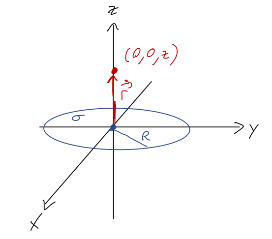
Last time we found \( g_x = g_y = 0 \), both by symmetry and explicitly. Now let's move on to the non-zero part of the field, \( g_z \). Since we've already gone through the details of the setup for \( x \), it should be easy to see that
\[ \begin{aligned} g_z = -G \sigma \int_0^{2\pi} d\phi' \int_0^R d\rho' \frac{\rho' z}{(\rho'^2 + z^2)^{3/2}} \\ = -2\pi G \sigma z \int_0^R \frac{d\rho' \rho'}{(\rho'^2 + z^2)^{3/2}}. \end{aligned} \]
This is actually a very friendly integral for \( u \)-substitution! Let's pick \( u = \rho'^2 + z^2 \), which gives \( du = 2\rho' d\rho' \). Then
\[ \begin{aligned} g_z = -2\pi G \sigma z \int_{z^2}^{R^2 + z^2} \frac{du/2}{u^{3/2}} \\ = -\pi G \sigma z \left( \left. -\frac{2}{u^{1/2}} \right|_{z^2}^{R^2+z^2} \right) \\ = 2\pi G \sigma z \left( \frac{1}{\sqrt{R^2 + z^2}} - \frac{1}{|z|} \right). \\ \end{aligned} \]
We could replace the density \( \sigma \) with the total mass \( M \); since it's a two-dimensional density, we have \( M = \sigma \pi R^2 \). But there's no normalizing \( 1/M \) like there is for the center of mass, so for this calculation it's fine to just leave it in terms of \( \sigma \) in general.
Clicker Question
Given the result:
\[ \begin{aligned} g_z = 2\pi G \sigma z \left( \frac{1}{\sqrt{R^2 + z^2}} - \frac{1}{|z|} \right) \end{aligned} \]
Which way does the gravitational field point (i.e. what is the sign of \( g_z \)?)
A. \( \vec{g} \) always points up (\( g_z > 0 \)).
B. \( \vec{g} \) always points down (\( g_z < 0 \)).
C. \( \vec{g} \) always points towards the disk.
D. \( \vec{g} \) always points away from the disk.
E. It points down for positive \( z \), and this formula isn't valid for negative \( z \).
Answer: C
Since \( \sqrt{R^2 + z^2} > |z| \) always, we have (1/big - 1/small) so the whole field is proportional to \( -z \). This makes sense - the direction of the field, and thus of the gravitational force \( \vec{F} = m\vec{g} \) on a test mass, always points towards the disk at \( z=0 \).
Clicker Question
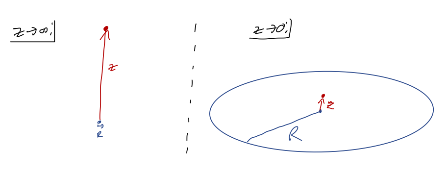
What is the correct expression for the field as we get very close to the disk, \( z \rightarrow 0 \)?
A. \( g_z = 2\pi G \sigma \frac{z}{R} \)
B. \( g_z = -2\pi G \sigma \)
C. \( g_z = \pm 2\pi G \sigma \), with \( - \) for \( z > 0 \)
D. \( g_z = \pm 2\pi G \sigma \frac{z}{R} \), with \( + \) for \( z > 0 \)
E. \( g_z = \pm 2\pi G \sigma \frac{z}{R} \), with \( - \) for \( z > 0 \)
Answer: C
As \( z \rightarrow 0 \), approaching the disk, we have
\[ \begin{aligned} g_z \rightarrow 2\pi G \sigma z \left( \frac{1}{R} - \frac{1}{|z|} \right) \approx -2\pi G \sigma \frac{z}{|z|} \end{aligned} \]
which is a constant - the fraction \( z/|z| \) just gives us either +1 above the disk or -1 below it, ensuring that the field points towards the disk. This makes sense: if we get arbitrarily close to the disk, from our perspective it will look just like standing on a very large flat surface, from which we would expect just a constant gravity field pointing "down".
The other limit to consider is \( z \rightarrow \infty \). This means that \( z \gg R \), which we can use to series expand the first term in the field:
\[ \begin{aligned} \frac{1}{\sqrt{R^2 + z^2}} = \frac{1}{|z|} \frac{1}{\sqrt{1 + (R/z)^2}} \end{aligned} \]
Let's use the binomial formula to expand,
\[ \begin{aligned} (1+z)^n = 1 + nz + \frac{n(n-1)}{2} z^2 + ... \end{aligned} \]
which leads to, just keeping the first two terms,
\[ \begin{aligned} \frac{1}{\sqrt{R^2 + z^2}} \approx \frac{1}{|z|} \left(1 - \frac{R^2}{2z^2} + ... \right) \end{aligned} \]
The \( 1/|z| \) terms cancel off, and we're left with
\[ \begin{aligned} g_z \rightarrow 2\pi G \sigma \frac{z}{|z|} \left( -\frac{R^2}{2z^2} + ... \right) \end{aligned} \]
Now it's useful to substitute in \( M = \pi R^2 \sigma \), which will absorb the \( R^2 \) factor and leave us with
\[ \begin{aligned} g_z \rightarrow -\frac{GM}{z^2} \frac{z}{|z|} \end{aligned} \]
or \( \vec{g} = -GM/z^2 \hat{r} \), along the \( z \)-axis. So in this limit, the leading dependence on \( R \) vanishes and we just recover the single point-particle form of the gravitational field! This makes a lot of sense: if we're really, really far away from the disk, then the fact that it's an extended object doesn't really matter - in fact, from far enough away we probably wouldn't be able to tell that it has any radius, we would just see a point.
Gravitational potential of extended objects
So far, we haven't really used the fact that gravity is a conservative force. In fact, being able to write a potential energy function \( U(\vec{r}) \) can actually save us a lot of work when dealing with extended objects! Recall that the potential energy for a single test mass \( m \) in the gravity field of a source mass \( M \) is
\[ \begin{aligned} U(r) = -\frac{GMm}{r}. \end{aligned} \]
What if we have multiple sources? I'll skip the detailed derivation, but the answer is that we can simply add the potential energies: for example, in the following situation
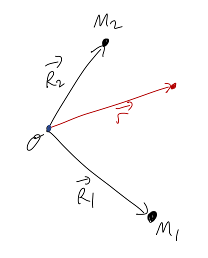
we just have
\[ \begin{aligned} U(\vec{r}) = -\frac{GM_1 m}{|\vec{r} - \vec{R}_1|} - \frac{GM_2 m}{|\vec{r} - \vec{R}_2|}. \end{aligned} \]
It's straightforward to see that taking \( \vec{F}_g = -\vec{\nabla} U \), where \( \vec{\nabla} \) is the gradient with respect to the \( \vec{r} \) coordinates, adding the potentials like this is equivalent to adding the gravitational forces together.
One more definition before we continue: like the force, the potential energy depends on the test mass \( m \), but in a very trivial way. It's often useful to factor out the \( m \) so we can calculate a function that only depends on the sources, which we can then apply to any test mass (or collection of test masses.) So just like we defined \( \vec{F}_g = m\vec{g} \), we now define the gravitational potential for a point source to be
\[ \begin{aligned} \Phi(r) = -\frac{GM}{r} \end{aligned} \]
so that \( U(r) = m\Phi(r) \). We can immediately see that \( \vec{g} = -\vec{\nabla} \Phi \), so this gives us another way to find the gravitational field. Potential is an unfortunate name for this quantity - keep in mind that \( \Phi \) is not a potential energy, it has the wrong units! This is completely analogous to the electric potential \( V(r) \), which is also not a potential energy - but the combination \( qV \) is.
Now if we have an extended object, as we saw before:
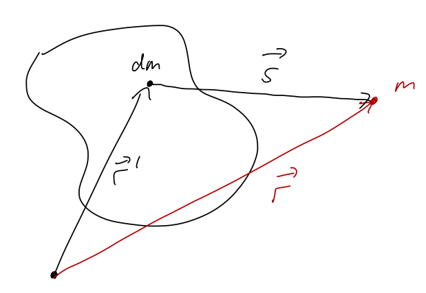
then the potential at position \( \vec{r} \) due to the infinitesmal source \( dm \) is
\[ \begin{aligned} d\Phi(\vec{r}) = -\frac{G dm}{s} = -\frac{G dm}{|\vec{r} - \vec{r}'|}, \end{aligned} \]
and thus the total potential is
\[ \begin{aligned} \Phi(\vec{r}) = -G \int \frac{dV' \rho(\vec{r}')}{|\vec{r} - \vec{r}'|}. \end{aligned} \]
This is much nicer to evaluate than the integrals we had to do for \( \vec{g} \)! Now we have no vector components to worry about - just a single scalar quantity. We can then take the gradient of our result (with respect to \( \vec{r} \)) to find the gravitational field \( \vec{g} \).
Let's do an example to see how this approach works in practice.
Example: gravitational potential of a thin ring
Consider a thin circular ring of mass \( M \) and radius \( a \), with uniform linear mass density \( \lambda \). What is the gravitational potential along the \( z \)-axis?
It's always a good idea to begin with a sketch:
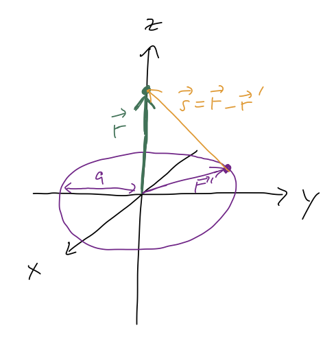
To make sure we're approaching the potential integral the right way, let's start by setting up the simpler integral for the total mass of the ring:
\[ \begin{aligned} M = \int dm = \int ds' \lambda(\vec{r}'). \end{aligned} \]
The coordinate setup will be the same as for the potential, but the result is much easier. Once again, cylindrical coordinates look like a good match for this problem. Given the radius \( a \) of the ring, we can write an infinitesmal length segment along the ring as
\[ \begin{aligned} ds' = a d\phi' \end{aligned} \]
using the definition of arc length for a circle. (This can also be thought of as a parametrization of the "path" around the circle, similar to what we did for line integration.) Plugging back in to the integral, we have
\[ \begin{aligned} M = \int_0^{2\pi} d\phi' a \lambda = 2\pi a \lambda \end{aligned} \]
or \( \lambda = M / (2\pi a) \). This makes sense, since \( 2\pi a \) is the circumference of the circle, and dividing the total mass by the length should give us the density when it's uniform (as it is here.)