We started with a clicker question on complex numbers:
Clicker Question
Which answer below is equal to \( \frac{1}{1-i} \)?
A. \( e^{i\pi/4} \)
B. \( \frac{1}{2} e^{i\pi/4} \)
C. \( \frac{1}{2} e^{-i\pi/4} \)
D. \( \frac{1}{\sqrt{2}} e^{i\pi/4} \)
E. \( \frac{1}{\sqrt{2}} e^{-i\pi/4} \)
Answer: D
There are two ways to solve this problem. We'll start with Euler's formula, which I promised would make things easier! Using
\[ \begin{aligned} 1-i = |z| (\cos(\theta) + i \sin (\theta)) \end{aligned} \]
we first see that we're looking for an angle where \( \cos \) and \( \sin \) are equal in magnitude (which means \( \pi/4, 3\pi/4, 5\pi/4 \), or \( 7\pi/4 \).) Since \( \cos \) is positive while \( \sin \) is negative, this points us to quadrant IV, so \( \theta = 7\pi/4 \) - I'll use \( \theta = -\pi/4 \) equivalently. Meanwhile, the complex magnitude is
\[ \begin{aligned} |z| = \sqrt{1^2 + (-1)^2} = \sqrt{2} \end{aligned} \]
so we have
\[ \begin{aligned} 1-i = \sqrt{2} e^{-i\pi/4}. \end{aligned} \]
If you prefer to just plug in to formulas, we can also get this with \( \tan^{-1}(y/x) = \theta \), but we still have to be careful about quadrants. In fact, an even simpler way to find this result would probably have been to just draw a sketch in the complex plane.
Inverting this is easy: we get
\[ \begin{aligned} \frac{1}{1-i} = \frac{1}{\sqrt{2}} e^{i\pi/4} = \frac{1}{2} (1+i), \end{aligned} \]
matching answer D. You can easily verify from the second form here that multiplying this by \( (1-i) \) gives 1.
The second way to solve this problem without polar angles is to multiply through the numerator and denominator by the complex conjugate:
\[ \begin{aligned} \frac{1}{1-i} = \frac{1+i}{(1-i)(1+i)} \end{aligned} \]
This gives us a difference of squares in the denominator which will get rid of the imaginary part:
\[ \begin{aligned} \frac{1+i}{(1-i)(1+i)} = \frac{1+i}{1^2 - i^2} = \frac{1}{2} (1+i) \end{aligned} \]
Now we have to convert this back to polar form to compare to the answers above: it should be easy to see that
\[ \begin{aligned} 1+i = \sqrt{2} e^{i\pi/4} \end{aligned} \]
leading us to D.
Back to Euler's formula itself: we can invert the formula to find useful equations for \( \cos \) and \( \sin \). I'll leave it as an exercise to prove the following identities:
\[ \begin{aligned} \cos \theta = \frac{1}{2} (e^{i\theta} + e^{-i\theta}) \\ \sin \theta = \frac{-i}{2} (e^{i\theta} - e^{-i\theta}) \end{aligned} \]
(These are, incidentally, extremely useful in simplifying integrals that contain products of trig functions. We'll see this in action later on!)
Complex solutions to the SHO
Back to the SHO equation,
\[ \begin{aligned} \ddot{x} = -\omega^2 x \end{aligned} \]
The minus sign in the equation is very important. We saw before that for equilibrium points that are unstable, the equation of motion we found near the equilibrium was \( \ddot{x} = +\omega^2 x \). This equation has solutions that are exponential in \( t \), moving rapidly away from equilibrium.
But now that we've introduced complex numbers, we can also write an exponential solution to the SHO equation. Notice that if we take \( x(t) = e^{i\omega t} \), then
\[ \begin{aligned} \ddot{x} = \frac{d}{dt} (i \omega e^{i \omega t}) = (i \omega)^2 e^{i \omega t} = -\omega^2 e^{i\omega t} \end{aligned} \]
and so this satisfies the equation. So does the function \( e^{-i\omega t} \) - the extra minus sign cancels when we take two derivatives. These are independent functions, even though they look very similar; there is no constant we can multiply \( e^{i\omega t} \) by to get \( e^{-i \omega t} \). Thus, another way to write the general solution is
\[ \begin{aligned} x(t) = C_1 e^{i\omega t} + C_2 e^{-i \omega t}. \end{aligned} \]
Now, this is a physics class (and we're not doing quantum mechanics!), so obviously the position of our oscillator \( x(t) \) always has to be a real number. However, by introducing \( i \) we have found a solution for \( x(t) \) valid over the complex numbers. The only way that this can make sense is if choosing physical (i.e. real) initial conditions for \( x(0) \) and \( \dot{x}(0) \) gives us an answer that stays real for all time; otherwise, we've made a mistake somewhere.
Let's see how this works by imposing those initial conditions: we have
\[ \begin{aligned} x(0) = x_0 = C_1 + C_2 \\ v(0) = v_0 = i\omega (C_1 - C_2) \end{aligned} \]
This obviously only makes sense if \( C_1 + C_2 \) is real and \( C_1 - C_2 \) is pure imaginary - which means the coefficients \( C_1 \) and \( C_2 \) have to be complex! (This isn't a surprise, since we asked for a solution over complex numbers.) If we write
\[ \begin{aligned} C_1 = x + iy \end{aligned} \]
then the conditions above mean that we must have \( C_2 = x - iy \) so the real and imaginary parts cancel appropriately. In other words, we must have a general solution of the form
\[ \begin{aligned} x(t) = C_1 e^{i\omega t} + C_1^\star e^{-i\omega t}. \end{aligned} \]
This might look confusing, since we now seemingly have one arbitrary constant instead of the two we need. But it's one arbitrary complex number, which is equivalent to two arbitrary reals. In fact, we can finish plugging in our initial conditions to find
\[ \begin{aligned} C_1 = \frac{x_0}{2} - \frac{iv_0}{2\omega} \end{aligned} \]
so both of our initial conditions are indeed separately contained in the single constant \( C_1 \).
Now, if we look at the latest form for \( x(t) \), we notice that the second term is exactly just the complex conjugate of the first term. Recalling the definition of the real part as
\[ \begin{aligned} {\rm Re}(z) = \frac{1}{2} (z + z^\star), \end{aligned} \]
we can rewrite this more compactly as
\[ \begin{aligned} x(t) = 2\ {\rm Re}\ (C_1 e^{i\omega t}). \end{aligned} \]
This is nice, because now \( x(t) \) is manifestly always real! (But remember that we did not just arbitrarily "take the real part" to enforce this; it came out of our initial conditions. It's not correct to solve over the complex numbers and then just ignore half the solution!)
At this point, let's try to compare back to our trig-function solutions; we know they're hiding in there somehow, thanks to Euler's formula.
Let's verify that the real part written above gives back the previous general solution. The best way to do this is to expand our all the complex numbers into real and imaginary components, do some algebra, and then just read off what the real part of the product is. Let's substitute in using both \( C_1 \) from above and Euler's formula:
\[ \begin{aligned} x(t) = 2\ {\rm Re}\ \left[ \left( \frac{x_0}{2} - \frac{iv_0}{2\omega} \right) \left( \cos (\omega t) + i \sin (\omega t) \right) \right] \end{aligned} \]
Pulling the \( 2 \) in from the front and then multiplying through,
\[ \begin{aligned} x(t) = {\rm Re}\ \left[ x_0 \cos(\omega t) + ix_0 \sin (\omega t) - \frac{iv_0}{\omega} \cos (\omega t) + \frac{v_0}{\omega} \sin (\omega t) \right] \\ = {\rm Re}\ \left[ x_0 \cos (\omega t) + \frac{v_0}{\omega} \sin (\omega t) + i (...) \right] \\ = x_0 \cos (\omega t) + \frac{v_0}{\omega} \sin (\omega t) \end{aligned} \]
just ignoring the imaginary part. So indeed, this is exactly the same as our previous solution, just in a different form!
This is a nice confirmation, but the fact that \( C_1 \) is complex makes it a little non-obvious what the real and imaginary parts look like. We can fix that by rewriting it in polar notation. If I suggestively define
\[ \begin{aligned} C_1 = \frac{A}{2} e^{-i\delta}, \end{aligned} \]
then we have
\[ \begin{aligned} x(t) = {\rm Re}\ (A e^{-i\delta} e^{i\omega t}) = A\ {\rm Re}\ (e^{i(\omega t - \delta)}) \end{aligned} \]
pulling the real number \( A \) out of the real part. Now taking the real part of the combined complex exponential is easy: it's just the cosine of the argument,
\[ \begin{aligned} x(t) = A \cos (\omega t - \delta), \end{aligned} \]
exactly matching the other form of the SHO solution we wrote down before. (Notice: no need for trig identities this time! Complex exponentials are a very powerful tool for simplfying expressions involving trig functions.)
I'm going to completely skip over the two-dimensional oscillator; as we emphasized before, one-dimensional motion is special in terms of what we can learn from considering energy conservation, and similarly the SHO is especially useful in one dimension. Of course, the idea of expanding around equilibrium points is very general, but it will not just give you the 2d or 3d SHO equation that Taylor studies in (5.3). In general, you will end up with a coupled harmonic oscillator, the subject of chapter 11.
We can see what happens by just considering the seemingly simple example of a mass on a spring connected to the origin in two dimensions. If the equilibrium (unstretched) length of the spring is \( r_0 \), then
\[ \begin{aligned} \vec{F} = -k(r- r_0) \hat{r} \end{aligned} \]
or expanding in our two coordinates, using \( r = \sqrt{x^2 + y^2} \) and \( \hat{r} = \frac{1}{r} (x\hat{x} + y\hat{y}) \),
\[ \begin{aligned} m \ddot{x} = -kx (1 - \frac{r_0}{\sqrt{x^2 + y^2}}) \\ m \ddot{y} = -ky (1 - \frac{r_0}{\sqrt{x^2 + y^2}}) \end{aligned} \]
These are much more complicated than the regular SHO, and indeed we see they are coupled: both \( x \) and \( y \) appear in both equations. The regular two-dimensional SHO appears when \( r_0 = 0 \), and we just get two nice uncoupled SHO equations; but as I said, this is a special case, so I'll just let you read about it in Taylor.
The damped harmonic oscillator
For expanding around equilibrium, the SHO is all we need, and we've solved it thoroughly at this point. However, it turns out there's a lot of interesting physics and math in variations of the harmonic oscillator that have nothing to do with equilibrium expansion or energy conservation.
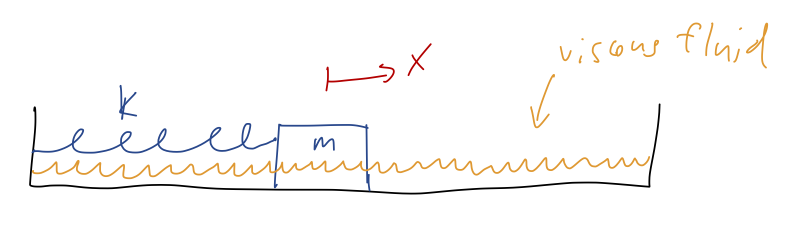
We'll begin our study with the damped harmonic oscillator. Damping refers to energy loss, so the physical context of this example is a spring with some additional non-conservative force acting. Specifically, what people usually call "the damped harmonic oscillator" has a force which is linear in the speed, giving rise to the equation
\[ \begin{aligned} m \ddot{x} = - b\dot{x} - kx. \end{aligned} \]
The new force is the familiar linear drag force, so we can imagine this to be the equation describing a mass on a spring which is sliding through a high-viscosity fluid, like molasses:
As Taylor observes, another very important instance of this equation is the LRC circuit, which contains an inductor, a resistor, and a capacitor in series. The differential equation for the charge in such a circuit is
\[ \begin{aligned} L\ddot{Q} + R\dot{Q} + \frac{Q}{C} = 0. \end{aligned} \]
Since this is not a circuits class I won't dwell on this example, but I point it out for those of you who might be more familiar with circuit equations.
Let's rearrange the equation of motion slightly and divide out by the mass, as we did for the SHO:
\[ \begin{aligned} \ddot{x} + 2\beta \dot{x} + \omega_0^2 x = 0 \end{aligned} \]
where
\[ \begin{aligned} \beta = \frac{b}{2m},\ \ \omega_0 = \sqrt{\frac{k}{m}}, \end{aligned} \]
using the conventional notation for this problem. The frequency \( \omega_0 \) is called the natural frequency; as we can see, it is the frequency at which the system would oscillate if we removed the damping term by setting \( b=0 \). The other constant \( \beta \) is called the damping constant, and it is proportional to the strength of the drag force. \( \beta \) has the same units as \( \omega_0 \), i.e. frequency or 1/time.
Once again, we have a linear, second-order, homogeneous ODE, so we just need to find two independent solutions to put together. Unfortunately, it's a little harder to guess what the solutions will be just by inspection this time. Taylor uses the first method most physicists will reach for - guess and check, here guessing a complex exponential form. This sort of works, but in the special case \( \beta = \omega_0 \) (which we do want to cover) guess and check is much harder to use.
There is a more systematic way to find the answer, using the language of linear operators (as covered in Boas 8.5.) First of all, an operator is a generalized version of a function: it's a map that takes an input to an output based on some specific rules. The derivative \( d/dt \) can be thought of as an operator, which takes an input function and gives us back an output function. The "linear" part refers to operators that follow two simple rules:
\( \frac{d}{dt} (f(t) + g(t)) = \frac{df}{dt} + \frac{dg}{dt} \)
\( \frac{d}{dt} (a f(t)) = a \frac{df}{dt} \)
We already know that these are both true for \( d/dt \). What this means is that we can do algebra on the derivative operator itself. For example, using these properties we can write
\[ \begin{aligned} \frac{d^2f}{dt^2} + 3\frac{df}{dt} = 0 \Rightarrow \frac{d}{dt} \left( \frac{d}{dt} + 3 \right) f(t) = 0 \end{aligned} \]
or adopting the useful shorthand that \( D \equiv d/dt \),
\[ \begin{aligned} D (D+3) f(t) = 0 = (D+3) D f(t). \end{aligned} \]
On the last line, I re-ordered the two derivative terms. But this reordering is very useful, because it shows that there are two ways to satisfy the equation: both
\[ \begin{aligned} D f(t) = 0 \end{aligned} \]
and
\[ \begin{aligned} (D+3) f(t) = 0 \end{aligned} \]
will lead to solutions to the differential equation. Even better, the two solutions we get will be linearly independent (I won't prove this, see Boas), which means that solving each of these simple first-order equations immediately gives us the general solution to the original equation!
This gives us a very useful method to solve a whole class of second-order linear ODEs:
Rewrite the ODE in the form \( (aD^2 + bD + c) f = 0 \).
Solve for the roots of the auxiliary equation, \( (aD^2 + bD + c) = 0 = (D - r_1) (D - r_2) \)
Obtain the general solution from the solutions of \( (D-r_1) f = 0 \) and \( (D - r_2) f = 0 \).
Here I've assumed a homogeneous ODE, i.e. the right-hand side is zero. We can use the same method for non-homogeneous equations, but there's an extra step in that case: we have to add a particular solution, as we saw in the first-order case. Also, it's very important above that the constants are constant - in other words, if \( D = d/dt \), then \( a,b,c \) must all be independent of \( t \) or else the reordering trick doesn't work (it's easy to see that, for example, \( D (D+t) \) is not equal to \( (D+t) D \).)
Now let's use this method on the damped harmonic oscillator. Our ODE looks like
\[ \begin{aligned} \ddot{x} + 2\beta \dot{x} + \omega_0^2 x = 0 \end{aligned} \]
which we can rewrite as
\[ \begin{aligned} (D^2 + 2\beta D + \omega_0^2) x(t) = 0. \end{aligned} \]
To find the roots of the auxiliary equation, we can just use the quadratic formula:
\[ \begin{aligned} r_{\pm} = -\beta \pm \sqrt{\beta^2 - \omega_0^2}. \end{aligned} \]
The individual solutions, then, solve the first-order equations
\[ \begin{aligned} (D - r_{\pm}) x = 0, \end{aligned} \]
which we recognize as simple exponential solutions,
\[ \begin{aligned} x(t) \propto e^{r_{\pm} t}. \end{aligned} \]
Thus, our general solution is:
\[ \begin{aligned} x(t) = C_1 e^{r_+ t} + C_2 e^{r_- t} \\ = C_1 e^{-\beta t + \sqrt{\beta^2 - \omega_0^2} t} + C_2 e^{-\beta t - \sqrt{\beta^2 - \omega_0^2} t} \\ = e^{-\beta t} \left( C_1 e^{\sqrt{\beta^2 - \omega_0^2} t} + C_2 e^{-\sqrt{\beta^2 - \omega_0^2}t} \right). \end{aligned} \]
(There is one subtlety here: if \( r_+ = r_- \), then we have actually only found one solution. I'll return to this case a little later.)
If we plug in \( \beta = 0 \) as a check, then we get \( \sqrt{-\omega_0^2} t = i\omega_0 t \) inside both of the exponentials in the second factor, giving back our undamped SHO solution as it should.