Last time, we ended on the general solution to the damped SHO equation:
\[ \begin{aligned} x(t) = e^{-\beta t} \left( C_1 e^{\sqrt{\beta^2 - \omega_0^2} t} + C_2 e^{-\sqrt{\beta^2 - \omega_0^2}t} \right). \end{aligned} \]
It should be obvious from looking at this that the relative size of \( \beta \) and \( \omega_0 \) will be very important in the qualitative behavior of these solutions: the exponentials inside the parentheses can be either real or imaginary as we change \( \beta \) relative to \( \omega_0 \). Let's go through the possibilities.
Damping strength and behavior of the damped SHO
Underdamped motion
Since we already know what happens at \( \beta = 0 \), let's start with small \( \beta \) and turn the strength of the force up from there. (\( \beta \) is dimensionless, so by "small \( \beta \)" I of course mean "small \( \beta/\omega_0 \).") In particular, as long as \( \beta < \omega_0 \), the combination \( \beta^2 - \omega_0^2 \) under the roots will always be negative. We define a new frequency \( \omega \) as follows:
\[ \begin{aligned} \sqrt{\beta^2 - \omega_0^2} = i \sqrt{\omega_0^2 - \beta^2} = i \omega. \end{aligned} \]
(Taylor calls this "\( \omega_1 \)", but the subscript 1 seems weird and confusing to me, so I'm deviating from his notation a little.) With this definition, we have for the overall solution
\[ \begin{aligned} x(t) = e^{-\beta t} \left(C_1 e^{i\omega t} + C_2 e^{-i\omega t} \right), \end{aligned} \]
or doing the same trick to combine the trig functions as before,
\[ \begin{aligned} x(t) = Ae^{-\beta t} \cos (\omega t - \delta). \end{aligned} \]
So we once again have an oscillating solution, almost the same as the SHO, except the amplitude dies off exponentially as \( e^{-\beta t} \). If we plot this, we can imagine an exponential "envelope" given by \( \pm Ae^{-\beta t} \), with the actual solution oscillating back and forth between the sides of the envelope:
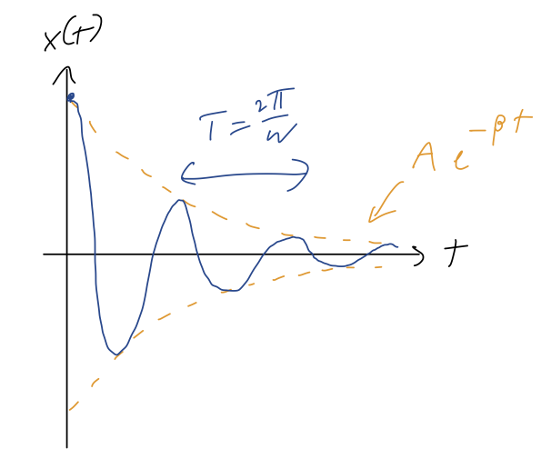
The solution above corresponds to releasing the oscillator at rest from some initial displacement. Note that this is no longer periodic, but the distance between maxima or minima within the envelope is still \( \tau = 2\pi / \omega \). If \( \beta \ll \omega_0 \), then we notice that \( \omega \approx \omega_0 \), so for very small damping the oscillation frequency is roughly the same as the natural oscillation. As the damping increases, the frequency of oscillation decreases (the peaks get further apart.)
Clicker Question
For the damped SHO released from rest with \( \beta < \omega_0 \), where does \( v(t) \) reach its maximum value \( v_{\rm max} \)?
A. Just before reaching \( x=0 \)
B. Just after reaching \( x=0 \)
C. Precisely at \( x=0 \)
D. It depends on other information.
Answer: A
There are two ways to argue this: using physics, or using math. Physics explanation first: let's think about the forces acting on our oscillator. We have
\[ \begin{aligned} \ddot{x} = -2\beta \dot{x} - \omega_0^2 x \end{aligned} \]
and the terms on the RHS are the two forces: the drag force and the spring force. Now let's think about the direction of these forces. When we release the oscillator at \( x_0 \) from rest, the drag force is initially zero, whereas the spring force gives a negative acceleration \( \ddot{x} < 0 \). This motion leads to a negative speed \( \dot{x} < 0 \), which means the drag force is positive - reducing the acceleration.
The maximum speed \( v_{\rm max} \) will then occur at the precise moment where \( \ddot{x} = 0 \), after which the sign of \( \ddot{x} \) changes and the mass starts to slow down again. But this can't be at \( x = 0 \)! For \( \ddot{x} = 0 \), the two forces have to cancel out, but at \( x=0 \) the spring force is zero. The drag force at \( x=0 \) is positive, so the oscillator is already slowing down; therefore, \( \ddot{x} = 0 \) (and thus \( v_{\rm max} \)) must have occurred before \( x=0 \), option A.
For the math version of the answer, we just take our solution from above and take a derivative:
\[ \begin{aligned} \dot{x}(t) = -\beta A e^{-\beta t} \cos (\omega t - \delta) - \omega A e^{-\beta t} \sin(\omega t - \delta) \end{aligned} \]
and then another derivative to get acceleration (or equivalently, to find where this function is extremized):
\[ \begin{aligned} \ddot{x}(t) = A e^{-\beta t} \left[ \beta^2 \cos(\omega t - \delta) + 2 \omega \beta \sin(\omega t - \delta) - \omega^2 \cos(\omega t - \delta) \right] \end{aligned} \]
Now, the point where \( x(t) = 0 \) is given by \( \cos(\omega t - \delta) = 0 \), which means that at the same time \( \sin(\omega t - \delta) \) is either \( +1 \) or \( -1 \). To decide which is which, we note that at \( t=0 \) we must have \( x > 0 \), which means that \( \cos \) starts out positive. As the angle \( \omega t - \delta \) increases, the next place where cosine will cross zero is between the first and second quadrants, where sine is +1. Thus, at \( x=0 \),
\[ \begin{aligned} \ddot{x} = A e^{-\beta t} \left[ +2\omega \beta \right] \end{aligned} \]
which is positive - so it must have already flipped signs before \( x=0 \), and \( v_{\rm max} \) must have already happened.
By the way, notice what happens if we impose initial conditions on our simple harmonic oscillator solution:
\[ \begin{aligned} x(0) = A \cos(-\delta) \\ \dot{x}(0) = -A (\beta \cos (-\delta) + \omega \sin(-\delta)) \end{aligned} \]
We can see right away that this is going to be trickier than the regular SHO solution; in particular, it is not true that \( \delta = 0 \) gives us the solution starting from rest here! Using some trig identities, this leads to the set of equations
\[ \begin{aligned} x(0) = A \cos \delta \\ \dot{x}(0) = -A \beta \cos \delta \left[1 - \frac{\omega}{\beta} \tan \delta \right]. \end{aligned} \]
This gets messy to solve, but for the specific case of starting from rest, \( \dot{x}(0) = 0 \) leads us to the simpler result
\[ \begin{aligned} 1 - \frac{\omega}{\beta} \tan \delta = 0 \Rightarrow \delta = \tan^{-1} \left( \frac{\omega}{\beta} \right) = \tan^{-1} \left( \frac{\sqrt{\omega_0^2 - \beta^2}}{\beta} \right) \end{aligned} \]
which we can plug in to for the phase shift, and then plug in to the first equation to find \( A \). I won't go further with this - you'd want to do it numerically for a given oscillator, the general case isn't very enlightening. But I wanted to point out that \( A \) and \( \delta \) don't have quite the same simple interpretations anymore for the damped oscillator.
Overdamped motion
Let's move on to the case where \( \beta > \omega_0 \) - exact equality is tricky, so we'll do that last. In this case, all of the exponentials stay real, and we have
\[ \begin{aligned} x(t) = C_1 e^{-(\beta - \sqrt{\beta^2 - \omega_0^2}) t} + C_2 e^{-(\beta + \sqrt{\beta^2 - \omega_0^2}) t}. \end{aligned} \]
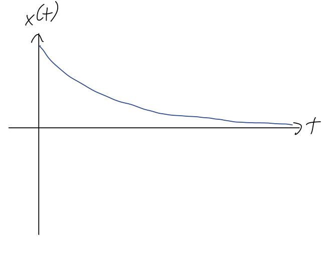
Since \( \sqrt{\beta^2 - \omega_0^2} < \beta \) given our assumptions, both terms decay exponentially in time, and there's no oscillation at all. Here's a sketch of this solution:
It's instructive to factor out the first exponential term completely from our solution:
\[ \begin{aligned} x(t) = e^{-(\beta - \sqrt{\beta^2 - \omega_0^2}) t} \left( C_1 + C_2 e^{-2\sqrt{\beta^2 - \omega_0^2} t}\right). \end{aligned} \]
As \( t \) increases, the second term here is negligible for the long-term behavior of the system, unless we have \( C_1 = 0 \). Let's match initial conditions to see what that would require:
\[ \begin{aligned} x_0 = x(0) = C_1 + C_2 \\ v_0 = \dot{x}(0) = -(\beta - \sqrt{\beta^2 - \omega_0^2}) C_1 - (\beta + \sqrt{\beta^2 - \omega_0^2}) C_2 \end{aligned} \]
We can solve this for \( C_1 = 0 \), and a bit of algebra reveals that it requires a specific relationship between \( v_0 \) and \( x_0 \),
\[ \begin{aligned} \frac{v_0}{x_0} = -(\beta + \sqrt{\beta^2 - \omega_0^2}). \end{aligned} \]
In particular, the minus sign tells us that this is only possible if \( v_0 \) and \( x_0 \) are in opposite directions. Aside from this rather special case, we can in general ignore the \( C_2 \) term completely at large \( t \), finding that
\[ \begin{aligned} x(t) \rightarrow C_1 e^{-\alpha t} \end{aligned} \]
defining the decay parameter \( \alpha \) as the coefficient in the exponential decay of the max amplitude at large \( t \), in this case
\[ \begin{aligned} \alpha = \beta - \sqrt{\beta^2 - \omega_0^2}. \end{aligned} \]
This solution exhibits some rather counterintuitive behavior: as we increase the strength of the damping force \( \beta \), the decay parameter \( \alpha \) actually becomes smaller, approaching \( \alpha = 0 \) as \( \beta \rightarrow \infty \)! To make sense of this, let's remember that the net force on our oscillator is
\[ \begin{aligned} F_{\rm net} = F_{\rm drag} + F_{\rm spring} = -2m\beta \dot{x} - k x \end{aligned} \]
Both forces push our object back towards the origin. But if \( \beta \) is extremely large, then there is an enormous force even if we try to move at a relatively small speed, so it will take much longer in time for us to actually get to the origin. We still get there eventually, because the \( -kx \) spring force always keeps pulling us to the origin as long as \( x \) is non-zero.
Critical damping
Finally, we come back to the third possibility, which is \( \beta = \omega_0 \). If we go back to our original solution, this gives us
\[ \begin{aligned} x(t) = C_1 e^{-(\beta - \sqrt{\beta^2 - \omega_0^2}) t} + C_2 e^{-(\beta + \sqrt{\beta^2 - \omega_0^2}) t} \rightarrow C_1 e^{-\beta t} + C_2 e^{-\beta t}. \end{aligned} \]
Now we only have one solution, repeated twice! This means our solution is suddenly incomplete: we need two independent functions to add together to have a general solution. To find a second solution, since this is clearly a special case, let's go back to the original differential equation and see what happens if \( \beta = \omega_0 \):
\[ \begin{aligned} \ddot{x} + 2 \beta \dot{x} + \beta^2 x = 0 \end{aligned} \]
Clearly \( e^{-\beta t} \) indeed works as a solution. To see the other one, let's go back to our linear operator language and notice that the auxiliary equation in this case is easy to factorize:
\[ \begin{aligned} \left( \frac{d^2}{dt^2} + 2\beta \frac{d}{dt} + \beta^2 \right) x(t) = 0 \end{aligned} \]
becomes
\[ \begin{aligned} \left( D + \beta \right) \left( D + \beta \right) x(t) = 0. \end{aligned} \]
One way that this equation can be satisfied is just if
\[ \begin{aligned} \left( D + \beta \right) x(t) = 0, \end{aligned} \]
which matches on to our solution \( e^{-\beta t} \). But the other possibility is that this combination isn't zero: let's call it
\[ \begin{aligned} \left( D + \beta \right) x(t) = u(t) \neq 0. \end{aligned} \]
Then we're left with another first-order ODE,
\[ \begin{aligned} \left( D + \beta \right) u(t) = 0. \end{aligned} \]
So \( u(t) = C e^{-\beta t} \), but now we have to work backwards a bit:
\[ \begin{aligned} \left( D + \beta \right) x(t) = C e^{-\beta t} \end{aligned} \]
We can use the general first-order solution in Boas to find the answer directly, but if you stare at this for a minute, you might think to try the following combination: if
\[ \begin{aligned} x(t) = C t e^{-\beta t} \end{aligned} \]
then
\[ \begin{aligned} \frac{dx}{dt} = C e^{-\beta t} - \beta C t e^{-\beta t} \end{aligned} \]
so the \( te^{-\beta t} \) will cancel out, matching the right-hand side. Thus, the general solution in this special case where \( \beta = \omega_0 \) is
\[ \begin{aligned} x(t) = C_1 e^{-\beta t} + C_2 t e^{-\beta t}. \end{aligned} \]
Once again, we see no oscillations - everything is pure exponential decay, but with an extra factor of \( t \) that only matters at small times. Once again as \( t \) becomes very large, the amplitude decays exponentially proportional to \( \beta \).
Let's summarize all of our solutions:
- If \( \beta < \omega_0 \), the system is said to be underdamped. Our solution takes the form
\[ \begin{aligned} x(t) = Ae^{-\beta t} \cos (\omega t - \delta), \end{aligned} \]
with oscillations, and the overall amplitude decaying with decay parameter \( \alpha = \beta \).
- If \( \beta = \omega_0 \), the system is critically damped. We have the funny solution we just found,
\[ \begin{aligned} x(t) = C_1 e^{-\beta t} + C_2 t e^{-\beta t}, \end{aligned} \]
with no oscillations and again the ampltiude at large times decaying exponentially with \( \alpha = \beta \).
- Finally, if \( \beta > \omega_0 \), the system is overdamped. In this case the general solution looks like
\[ \begin{aligned} x(t) = C_1 e^{-(\beta - \sqrt{\beta^2 - \omega_0^2}) t} + C_2 e^{-(\beta + \sqrt{\beta^2 - \omega_0^2}) t}. \end{aligned} \]
again pure exponential decay, but this time with decay parameter \( \alpha = \beta - \sqrt{\beta^2 - \omega_0^2} \), which goes to zero as \( \beta \) gets larger and larger.
We can sketch the size of the decay parameter vs. the damping parameter \( \beta \):
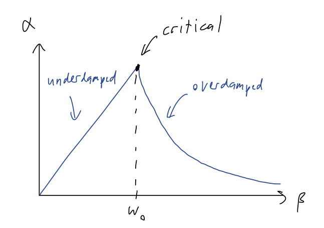
When designing a system that behaves like a damped oscillator, this tells us that it's actually optimal to tune \( \beta \) (or \( \omega_0 \)) so that the system is as close to critical as possible. A good example is shock absorbers in a car, which are designed to damp out the oscillations transferred from the road to the passengers.