Let's finish up our particular solution for sinusoidal driving. Putting everything back together, our particular solution becomes
\[ \begin{aligned} x_p(t) = A e^{-i\Delta} e^{i\omega t}. \end{aligned} \]
with
\[ \begin{aligned} A = \frac{F_0/m}{\sqrt{\omega_0^2 - \omega^2)^2 + 4\beta^2 \omega^2}} \end{aligned} \]
and
\[ \begin{aligned} \tan \delta = \frac{2\beta \omega}{\omega_0^2 - \omega^2} \end{aligned} \]
Once again, this has to be real since it's a position. We've seen this before for the regular damped oscillator: once we are careful about plugging in initial conditions, the solution actually is real even though it looks complex. But this is the particular solution, so the initial conditions don't affect it! So how do we make sure it's real?
The answer is that the particular solution is determined by the driving term, and the driving force we solved with is complex:
\[ \begin{aligned} F(t) = F_0 e^{-i \delta_0} e^{i\omega t}. \end{aligned} \]
Obviously in a real physical system, \( F(t) \) has to be real - which it currently is not. The good news is that this is easy to fix; if we add the complex conjugate, then we'll get a manifestly real force, i.e.
\[ \begin{aligned} {\rm Re} [F(t)] = \frac{1}{2} F_0 \left( e^{i(\omega t - \delta_0)} + e^{-i(\omega t - \delta_0)} \right) \\ = F_0 \cos (\omega t - \delta_0). \end{aligned} \]
The first term in the real part is the solution we just found; the second term is almost the same, but it requires making the substitutions \( \omega \rightarrow -\omega \) and \( \delta_0 \rightarrow -\delta_0 \). Using the equations for \( A \) and \( \tan \delta \) above, you should be able to convince yourself that these substitutions map \( A \rightarrow A \) and \( \delta \rightarrow -\delta \). Thus, the particular solution for the real force above becomes
\[ \begin{aligned} x_p(t) = \frac{1}{2} A \left[ e^{-i\Delta} e^{i\omega t} + e^{+i\Delta} e^{-i\omega t} \right] \\ = A \cos (\omega t - \delta_0 - \delta). \end{aligned} \]
(This relies on the fact that if we have a driving force that splits into two parts, we just add the particular solutions for each force individually - it's easy to prove that this gives the combined particular solution.)
To get a better feeling for the phase factors here, suppose that the driving force is purely cosine, i.e.
\[ \begin{aligned} F(t) = F_0 \cos (\omega t). \end{aligned} \]
Then \( \delta_0 = 0 \), and we find that the solution is \( A \cos(\omega t - \delta) \) - i.e. still a pure cosine, but phase shifted from the applied driving. Likewise, sinusoidal driving gives a sine-wave response:
\[ \begin{aligned} F(t) = F_0 \sin (\omega t) \Rightarrow x_p(t) = A \sin (\omega t - \delta). \end{aligned} \]
Let's look at another special case to try to get a better feeling for this solution. Suppose that we have pure cosine driving \( F(t) = F_0 \cos (\omega t \), and we're in the underdamped case, \( \beta < \omega_0 \). Then we can write the full solution with driving in the form
\[ \begin{aligned} x(t) = A \cos (\omega t - \delta) + A_1 e^{-\beta t} \cos (\omega_1 t - \delta_1) \end{aligned} \]
This is a little complicated-looking, but the second part of the solution is known as the transient; more important than the oscillation, it dies off exponentially as \( t \) increases. So although the short-time behavior will include both components, if we wait long enough, the transient term vanishes and we're just left with a simple oscillation at the driving frequency:
![]()
In fact, this is completely general: we know the critically damped and overdamped cases also die off exponentially with time, so those components are also transients. We find that no matter what \( \beta \) is, the long-term behavior of a driven damped oscillator is just simple oscillation at exactly the driving frequency.
Let's summarize what we've found. The key points to remember for sinusoidal (i.e. complex exponential) driving force \( F(t) = F_0 e^{i\omega t} \) are:
- The long-term behavior is oscillation of the form
\[ \begin{aligned} x(t) \rightarrow A \cos (\omega t - \delta) \end{aligned} \]
at exactly the same angular frequency \( \omega \) as the driving force. At shorter times there will be an additional transient behavior, with form depending on whether the system is over/underdamped.
- The motion of the system is phase shifted relative to the driving force, with phase shift given by
\[ \begin{aligned} \tan \delta = \frac{2\beta \omega}{\omega_0^2 - \omega^2}. \end{aligned} \]
- The amplitude of the system depends not just on the strength of the force, but also on the frequency of the driving, the natural frequency, and the damping constant:
\[ \begin{aligned} A = \frac{F_0/m}{\sqrt{(\omega_0^2 - \omega^2)^2 + 4\beta^2 \omega^2}}. \end{aligned} \]
Resonance
Now let's move on to talk about resonance, an interesting phenomenon which occurs in cases where the damping is relatively weak compared to both of the other frequencies, \( \beta \ll \omega, \omega_0 \). Resonance can be thought of as something which occurs when we vary the frequency and look at the amplitude of oscillations. In fact, we can see the effect qualitatively just from the amplitude formula we found. The denominator is
\[ \begin{aligned} \sqrt{(\omega_0^2 - \omega^2)^2 + 4 \beta^2 \omega^2} \end{aligned} \]
If \( \beta \) is relatively small, then we see that whenever \( \omega \approx \omega_0 \), the denominator is close to zero, which means the amplitude will be very large. We can think of this as a phenomenon which occurs either when varying \( \omega \) or varying \( \omega_0 \), with both cases being appropriate for different physical systems:
As we've referred to before, an LRC circuit is a common example of a damped oscillator. When a radio station broadcasts its signal, it does so at a fixed frequency \( \omega \) - the radio signal is the driving force in the LRC case. To listen to the radio, you tune your radio to change \( \omega_0 \), by adjusting the resistance or capacitance of your radio circuit. So in this case, \( \omega \) is fixed and we should think about changing \( \omega_0 \).
On the other hand, a real-world mechanical system like a bridge might have a certain natural frequency \( \omega_0 \) which is not easily adjusted. However, a person walking across the bridge provides a driving force with adjustable frequency \( \omega \). So now we think of \( \omega_0 \) as fixed and imagine changing \( \omega \).
Since \( \omega \) appears twice in the denominator, the simpler case will be when we hold it fixed and vary \( \omega_0 \). But for small enough \( \beta \), the behavior (i.e. the phenomenon of resonance) will be the same in both cases.
Let's think about the small-\( \beta \) limit, although we have to be careful with how we expand: we want to avoid actually taking \( \beta \) all the way to zero. As long as \( \beta^2 \) is small compared to either \( \omega^2 \) or \( \omega_0^2 \), we see that the second term underneath the square root is always very small. Meanwhile, the first term will also become small if we let \( \omega_0 \rightarrow \omega \). Once both terms are small, the overall amplitude will become very large - diverging, in fact, if we really try to set \( \beta = 0 \).
Let's factor out a \( 1/\omega^2 \) from everything, resulting in
\[ \begin{aligned} A = \frac{F_0/m}{\omega^2 \sqrt{(1 - \omega_0^2 / \omega^2)^2 + 4 \beta^2 / \omega^2 }}. \end{aligned} \]
Now we series expand as \( \omega_0 / \omega \rightarrow 1 \). As usual, this is easier if we change variables: let's say that \( \omega_0 = \omega + \epsilon \). Then
\[ \begin{aligned} (1 - \omega_0^2 / \omega^2)^2 = (1 - (1 - \epsilon/\omega)^2)^2 = (1 - 1 + 2\epsilon/\omega - \epsilon^2/\omega^2)^2 \approx 4\epsilon^2/\omega^2 \end{aligned} \]
discarding higher-order terms in \( \epsilon \). Then series expanding with the binomial formula gives
\[ \begin{aligned} A = \frac{F_0/m}{\omega \sqrt{4\epsilon^2 + 4\beta^2}} \\ = \frac{F_0}{2\omega m} \left( \frac{1}{\beta} - \frac{\epsilon^2}{2\beta^3} + ...\right) \end{aligned} \]
So close to \( \omega_0 = \omega \), we have a local maximum amplitude of \( A = F_0 / (2m \omega \beta) \). Near this maximum, as we change \( \omega_0 \) slightly away from \( \omega \), the amplitude decreases quadratically. In fact, it's easy to see that this peak is the global maximum: any value of \( \omega_0 \) different from \( \omega \) gives a positive contribution to the denominator and makes \( A \) smaller.
Moving away from the peak, we see furthermore that as \( \omega_0 \rightarrow 0 \) the amplitude goes to a finite value,
\[ \begin{aligned} A(\omega_0 \rightarrow 0) \rightarrow \frac{F_0/m}{\omega^2 \sqrt{1 + 4\beta^2 / \omega^2}} \approx \frac{F_0}{m \omega^2} \end{aligned} \]
using the fact that we're in the weak-damping limit so \( \beta / \omega \) is small. This also tells us that this value of \( A \) is much smaller than the peak, again by one power of \( \beta / \omega \). Finally, going to large natural frequency, the \( \omega_0^4 \) term eventually dominates everything else, and we find
\[ \begin{aligned} A(\omega_0 \rightarrow \infty) \rightarrow \frac{F_0}{m \omega_0^2}, \end{aligned} \]
which dies off to zero as \( \omega_0 \) gets larger and larger. Now we have all the information we need to make a sketch of amplitude vs. natural frequency:
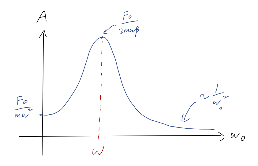
The large peak in the amplitude is called a resonance. Basically, we obtain a huge increase in the amplitude of oscillations as we tune the natural frequency \( \omega_0 \) close to the driving frequency \( \omega \). This effect is stronger when \( \beta \) is small: as \( \beta \) decreases, the peak amplitude becomes larger and the resonance becomes sharper (the width decreases.)
Now let's briefly consider the alternative situation, where \( \omega_0 \) is fixed and we are instead adjusting the driving frequency \( \omega \). This will be a lot messier if we try to series expand, but we know that we expect the same qualitative behavior: as the term \( \omega_0 - \omega \) vanishes in the denominator, the amplitude will become very large as long as the second term including \( \beta \) is relatively small. Instead of doing the full series expansion, let's use a derivative to find the position of the resonance peak. It will be easier to work with the squared amplitude for this:
\[ \begin{aligned} |A|^2 = \frac{F_0^2/m^2}{(\omega_0^2 - \omega^2)^2 + 4\beta^2 \omega^2} \end{aligned} \]
(it should be clear that the maximum of \( |A| \) is also the maximum of \( |A|^2 \).) We can take a derivative of the whole thing to find extrema, but maximizing \( |A|^2 \) is the same thing as minimizing the denominator alone, so let's just work with that directly:
\[ \begin{aligned} \frac{d}{d\omega} \left[ (\omega_0^2 - \omega^2)^2 + 4\beta^2 \omega^2 \right] = -4 \omega (\omega_0^2 - \omega^2) + 8\beta^2 \omega = 0 \end{aligned} \]
This has a solution at \( \omega = 0 \), but we know already that's not the right answer for the resonance peak. Dividing out the overall \( \omega \) leaves us with a quadratic equation,
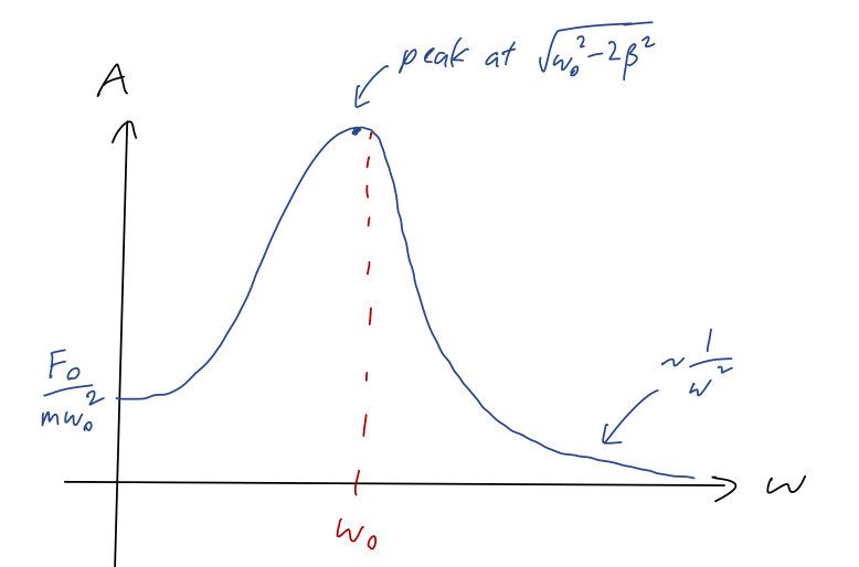
\[ \begin{aligned} 4 \omega^2 - 4\omega_0^2 + 8 \beta^2 = 0 \\ \omega = \sqrt{\omega_0^2 - 2\beta^2} \end{aligned} \]
taking the positive root since \( \omega \) has to be positive. This is close to \( \omega_0 \) for small \( \beta \), so this is definitely the location of the resonance peak! We notice that in this case, there's actually a small offset: the peak as a function of \( \omega \) is slightly to the left of \( \omega = \omega_0 \).
Clicker Question
What is the behavior of \( |A| \) at fixed \( \omega_0 \), as \( \omega \rightarrow \infty \)?
\[ \begin{aligned} |A| = \frac{F_0/m}{\sqrt{(\omega_0^2 - \omega^2)^2 + 4\beta^2 \omega^2}}. \end{aligned} \]
A. It goes to a constant value.
B. It goes to infinity.
C. It goes to zero, dying off as \( 1/\omega^2 \).
D. It goes to zero, dying off as \( 1/\omega \).
E. It goes to zero, dying off as some other power of \( \omega \) not given.
Answer: C
Since \( \omega_0 \) is being held fixed, we know that it will be negligible as \( \omega \) becomes larger and larger, which lets us make the replacement
\[ \begin{aligned} (\omega_0^2 - \omega^2)^2 \approx \omega^4. \end{aligned} \]
so for the denominator as a whole, we have
\[ \begin{aligned} A = \frac{F_0/m}{\sqrt{\omega^4 + 4\beta^2 \omega^2}} = \frac{F_0/m}{\omega^2 \sqrt{1 + 4\beta^2/\omega^2}} \sim \frac{1}{\omega^2} \end{aligned} \]
since no matter how strong the damping is, the second term \( 4\beta^2 / \omega^2 \) will be much less than 1 and so we can ignore it asymptotically. Thus, we find answer C.
Let's make another sketch here, using the behavior we just found; we'll also need to know what happens as \( \omega \rightarrow 0 \). In the latter case, we can just plug in directly and not even worry about expanding anything to find
\[ \begin{aligned} A(\omega \rightarrow 0) = \frac{F_0}{m\omega_0^2}. \end{aligned} \]
Thus, the sketch of amplitude for varying \( \omega \) looks like this:
If we plug back in the peak value into the amplitude formula, we find
\[ \begin{aligned} A = \frac{F_0/m}{\sqrt{(\omega_0^2 - (\omega_0^2 - 2\beta^2))^2 + 4\beta^2 (\omega_0^2 - 2\beta^2)}} \\ = \frac{F_0/m}{\sqrt{4 \beta^2 (\omega_0^2 - \beta^2)}} \approx \frac{F_0}{2m\omega_0 \beta} \end{aligned} \]
neglecting the extra term proportional to \( (\beta/\omega_0)^2 \). This is the same as in the case where we varied \( \omega_0 \).