The combination of the integral results we found last time and the Fourier series is incredibly powerful! Recall that the definition of the Fourier series representation of a function \( f(t) \) was
\[ \begin{aligned} f(t) = \sum_{n=0}^\infty \left[ a_n \cos(n \omega t) + b_n \sin (n \omega t) \right]. \end{aligned} \]
Suppose we want to know what the coefficient \( a_4 \) is. Thanks to the integral formulas we found above, if we integrate the entire series against the function \( \cos(4 \omega t) \), the integral will vanish for every term except precisely the one we want:
\[ \begin{aligned} \frac{2}{\tau} \int_{-\tau/2}^{\tau/2} f(t) \cos(4 \omega t) dt \\ = \frac{2}{\tau} \sum_{n=0}^\infty \left[ a_n \int_{-\tau/2}^{\tau/2} \cos (n \omega t) \cos (4 \omega t) dt + b_n \int_{-\tau/2}^{\tau/2} \sin(n \omega t) \cos (4 \omega t) dt \right] \\ = \sum_{n=0}^{\infty} \left[ a_n \delta_{n4} + b_n (0) \right] = a_4. \end{aligned} \]
In fact, we can now write down a general integral formula for all of the coefficients in the Fourier series:
\[ \begin{aligned} a_n = \frac{2}{\tau} \int_{-\tau/2}^{\tau/2} f(t) \cos(n \omega t) dt, \\ b_n = \frac{2}{\tau} \int_{-\tau/2}^{\tau/2} f(t) \sin(n \omega t) dt, \\ a_0 = \frac{1}{\tau} \int_{-\tau/2}^{\tau/2} f(t) dt, \\ b_0 = 0. \end{aligned} \]
The \( n=0 \) cases are special, and I've split them out: of course, \( b_0 \) is always multiplying the function \( \sin(0) = 0 \), so it doesn't matter what it is - we can just ignore it. As for \( a_0 \), it is a valid part of the Fourier series, but it corresponds to a constant offset. We find its value by just integrating the function \( f(t) \); this integral is zero for any of the trig functions, but just gives back \( \tau \) on the constant \( a_0 \) term.
Let's take a moment to appreciate the power of this result! To calculate a Taylor series expansion of a function, we have to compute derivatives of the function over and over until we reach the desired truncation order. These derivatives will generally become more and more complicated to deal with as they generate more terms with each iteration. On the other hand, for the Fourier series we have a direct and simple formula for any coefficient; finding \( a_{100} \) is no more difficult than finding \( a_1 \)! So the Fourier series is significantly easier to extend to very high order.
Example: the sawtooth wave
Let's do a concrete and simple example of a Fourier series decomposition. Consider the following function which is periodic but always linearly increasing (this is sometimes called the sawtooth wave):
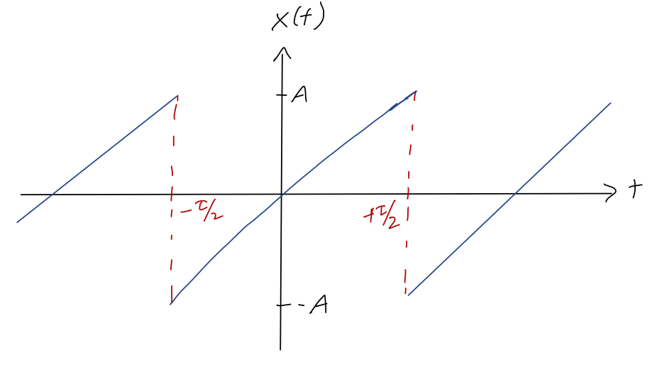
The equation describing this curve is
\[ \begin{aligned} x(t) = 2A\frac{t}{\tau},\ -\frac{\tau}{2} \leq t < \frac{\tau}{2} \end{aligned} \]
Let's find the Fourier series coefficients for this curve. Actually, we can save ourselves a bit of work if we think carefully first!
Clicker Question
What must be true about the Fourier series representation of the sawtooth wave?
\[ \begin{aligned} f(t) = a_0 + \sum_{n=1}^{\infty} [a_n \cos (n \omega t) + b_n \sin (n \omega t) ] \end{aligned} \]
A. All of the \( a_n \) are equal to zero.
B. All of the \( b_n \) are equal to zero.
C. All of the \( a_n \) are equal to zero, except for \( a_0 \).
D. All of the even \( a_n \) (\( a_0, a_2, a_4... \)) are equal to zero.
E. All of the even \( b_n \) (\( b_0, b_2, b_4... \)) are equal to zero.
Answer: A
There are a couple of ways to see that all of the \( a_n \) for \( n>0 \) have to vanish (we'll come back to \( a_0 \), which we generally have to think about separately.) First, we can just write out the integral for \( a_n \) using the definition of the sawtooth:
\[ \begin{aligned} a_n = \frac{4A}{\tau^2} \int_{-\tau/2}^{\tau/2} t \cos(n \omega t) dt. \end{aligned} \]
This integral is always zero, since \( \cos (n \omega t) \) is an even function for any \( n \), but \( t \) is odd. We could also argue this directly from the Fourier series by observing that the sawtooth function itself is odd (within a single period \( \tau \)); this means that its series should only contain odd functions, meaning the \( \cos(n \omega t) \) parts should all be zero.
As for \( a_0 \), if we used the second argument above then odd-ness of the sawtooth tells us \( a_0 = 0 \) too. If we used integrals, we can just write out the integral again to find
\[ \begin{aligned} a_0 = \frac{1}{\tau} \int_{-\tau/2}^{\tau/2} x(t) dt = \frac{1}{\tau} \int_{-\tau/2}^{\tau/2} \frac{2A}{\tau} t\ dt = 0. \end{aligned} \]
We can also read this off the graph: \( a_0 \) is just the average value of the function over a single period, which is clearly zero.
The above observation is something we should always look for when computing Fourier series: if the function to be expanded is odd, then all of the \( a_n \) will vanish (including \( a_0 \)), whereas if it is even, all the \( b_n \) will vanish instead.
On to the integrals we actually have to compute:
\[ \begin{aligned} b_n = \frac{4A}{\tau^2} \int_{-\tau/2}^{\tau/2} t \sin(n \omega t) dt \end{aligned} \]
This is a great candidate for integration by parts. Rewriting the integral as \( \int u dv \), we have
\[ \begin{aligned} u = t \Rightarrow du = dt \\ dv = \sin (n \omega t) dt \Rightarrow v = -\frac{1}{n \omega} \cos (n \omega t) \end{aligned} \]
and so
\[ \begin{aligned} \int u\ dv = uv - \int v\ du \\ = \left. -\frac{1}{n \omega} t \cos (n \omega t) \right|_{-\tau/2}^{\tau/2} + \frac{1}{n \omega} \int_{-\tau/2}^{\tau/2} \cos(n \omega t) dt \\ = -\frac{1}{n \omega} \left[ \frac{\tau}{2} \cos (n\pi) - \frac{-\tau}{2} \cos (-n\pi) \right] + \frac{1}{n^2 \omega^2} \left[ \sin (n \pi) - \sin (-n\pi) \right] \end{aligned} \]
The second term just vanishes since \( \sin(n\pi) = 0 \) for any integer \( n \). As for the first term, \( \cos(n\pi) \) is either \( +1 \) if \( n \) is even, or \( -1 \) if \( n \) is odd. Since \( \cos(-n\pi) = \cos(n\pi) \), we have the overall result
\[ \begin{aligned} \int u\ dv = -\frac{1}{n\omega} \left[ \frac{\tau}{2} (-1)^n + \frac{\tau}{2} (-1)^n \right] = -\frac{\tau}{n \omega} (-1)^n, \end{aligned} \]
or plugging the integral back into the Fourier coefficient formula,
\[ \begin{aligned} b_n = \frac{4A}{\tau^2} \int u\ dv = \frac{-4A \tau}{n \omega \tau^2} (-1)^n = -\frac{2A}{\pi n} (-1)^n = \frac{2A}{\pi n} (-1)^{n+1}, \end{aligned} \]
absorbing the overall minus sign at the very end. And now we're done - we have the entire Fourier series, all coefficients up to arbitrary \( n \) as a simple formula! Once again, you can appreciate how much easier it is to keep many terms before truncating in this case, compared to using a Taylor series. Plugging in some numbers to get a feel for this, the first few coefficients are
\[ \begin{aligned} b_1 = \frac{2A}{\pi},\ b_2 = -\frac{A}{\pi}, b_3 = \frac{2A}{3\pi}, b_4 = -\frac{A}{2\pi}, ... \end{aligned} \]
Importantly, the size of the coefficients is shrinking as \( n \) increases, due to the \( 1/n \) in our formula. Unlike the Fourier series, there is no automatic factor of \( 1/n! \) to help with convergence, so we should worry a little about the accuracy of truncating a Fourier series! It is, nevertheless, quite generic for the size of the Fourier series coefficients to die off in some way with \( n \). Remember that we're building a function up out of sines and cosines. Functions like \( \cos(n \omega t) \) with \( n \) very large are oscillating very, very quickly; if the function we're building up is relatively smooth, it makes sense that the really fast-oscillating terms won't be very important in modeling it.
Let's plug in some numbers and get a feel for how well our Fourier series does in approximating the sawtooth wave! Choosing \( A=1 \) and \( \omega = 2\pi \) (so \( \tau = 1 \)), here are some plots keeping the first \( m \) terms before truncating:

We can see that even as we add the first couple of terms, the approximation of the Fourier series curve to the sawtooth (the red line, plotted just for the region from \( -\tau/2 \) to \( \tau/2 \)) is already improving rapidly.
To visualize a bit better what's happening here, let's look at the three separate components of the final \( m=3 \) curve:
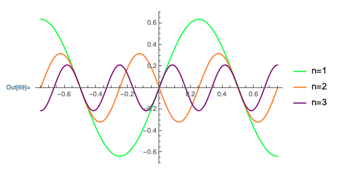
We clearly see that the higher-\( n \) components are getting smaller. If you compare the two plots, you can imagine "building up" the linear sawtooth curve one sine wave at a time, making finer adjustments at each step.
Of course, although \( m=3 \) might be closer to the sawtooth than you expected, it's still not that great - particularly near the edges of the region. Since we have an analytic formula, let's jump to a nice high truncation of \( m=50 \):

This is a remarkably good approximation - it's difficult to see the difference between the Fourier series and the true curve near the middle of the plot! At the discontinuities at \( \pm \tau/2 \), things don't work quite as well; we see the oscillation more clearly, and the Fourier series is overshooting the true amplitude by a bit. In fact, this effect (known as the Gibbs phenomenon) persists no matter how many terms we keep: there is a true asymptotic (\( n \rightarrow \infty \)) error in the Fourier series approximation whenever our function jumps discontinuously, so we never converge to exactly the right function.
The good news is that as we add more terms, this overshoot gets arbitrarily close to the discontinuity (the Gibbs phenomenon gets narrower), so we can still improve our approximation in that way. We'll always be stuck with this effect at the discontinuity, but of course real-world functions don't really have discontinuities, so this isn't really a problem in practice.
We could try to look at a plot of all of the 50 different sine waves that build up the \( m=50 \) sawtooth wave above, but it would be impossible to learn anything from the plot because it would be too crowded. Instead of looking at the whole sine waves, a different way to visualize the contributions is just to plot the coefficients \( |b_n| \) vs. \( n \):
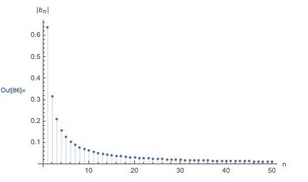
The qualitative \( 1/n \) behavior of the coefficients is immediately visible. This plot is sometimes known as a frequency domain plot, because the \( n \) on the horizontal axis is really a label for the size of the sine-function components with frequency \( n\omega \). If we didn't have a simple analytic formula and had to do the integrals for the \( a_n \) and \( b_n \) numerically, such a plot gives a simple way to check at a glance that the Fourier series is converging.
We'll only do this one example in lecture, but have a look in Taylor for a second example of finding the Fourier coefficients of a simple periodic function.
A useful analogy: Fourier series and vector spaces
Before we go back to our physics problem, a few more important thoughts on those crucial integral identities that let us pick off the Fourier series coefficients. Actually, I want to start with the new symbol we introduced above, the Kronecker delta symbol. We actually could have introduced this symbol all the way back at the beginning of the semester, when we were talking about vector coordinates. Remember that for a general three-dimensional coordinate system, we can expand any vector in terms of three unit vectors:
\[ \begin{aligned} \vec{a} = a_1 \hat{e}_1 + a_2 \hat{e}_2 + a_3 \hat{e}_3. \end{aligned} \]
The dot product of any two vectors is given by multiplying the components for each unit vector in turn:
\[ \begin{aligned} \vec{a} \cdot \vec{b} = (a_1 \hat{e}_1 + a_2 \hat{e}_2 + a_3 \hat{e}_3) \cdot (b_1 \hat{e}_1 + b_2 \hat{e}_2 + b_3 \hat{e}_3) \\ = a_1 b_1 + a_2 b_2 + a_3 b_3. \end{aligned} \]
What if we just take dot products of the unit vectors themselves, so \( a_i \) and \( b_i \) are either 1 or 0? We immediately see that we'll get 1 for the dot product of any unit vector with itself, and 0 otherwise, for example
\[ \begin{aligned} \hat{e}_1 \cdot \hat{e}_1 = 1, \\ \hat{e}_1 \cdot \hat{e}_3 = 0, \end{aligned} \]
and so on. The compact way to write this relationship is using the Kronecker delta again:
\[ \begin{aligned} \hat{e}_i \cdot \hat{e}_j = \delta_{ij}. \end{aligned} \]
This leads us to a technical math term that I didn't introduce before: the set of unit vectors \( {\hat{e}_1, \hat{e}_2, \hat{e}_3} \) form an orthonormal basis. "Basis" here means that we can write any vector at all as a combination of the unit vectors. Orthonormal means that all of the unit vectors are mutually perpendicular, and they all have length 1. Saying that the dot products of the unit vectors is given by the Kronecker delta is the same thing as saying they are orthonormal! Orthonormality is a useful property because it's what allows us to write the dot product in the simplest way possible.
Now let's imagine a fictitious space that has more than 3 directions, let's say some arbitrary number \( N \). We can use the same language of unit vectors to describe that space, and once again, it's most convenient to work with an orthonormal basis. It's really easy to extend what we've written above to this case! We find a set of vectors \( {\hat{e}_1, \hat{e}_2, ..., \hat{e}_N} \) that form a basis, and then ensure that they are orthonormal, which is still written in exactly the same way,
\[ \begin{aligned} \hat{e}_i \cdot \hat{e}_j = \delta_{ij}. \end{aligned} \]
We can then expand an arbitrary vector out in terms of unit-vector components,
\[ \begin{aligned} \vec{a} = a_1 \hat{e}_1 + a_2 \hat{e}_2 + ... + a_N \hat{e}_N. \end{aligned} \]
Larger vector spaces like this turn out to be very useful, even for describing the real world. You'll have to wait until next semester to see it, but they show up naturally in describing systems of physical objects, for example a set of three masses all joined together with springs. Since each individual object has three coordinates, it's easy to end up with many more than 3 coordinates to describe the entire system at once.
Let's wrap up the detour and come back to our current subject of discussion, which is Fourier series. This example is partly meant to help you think about the Kronecker delta symbol, but the analogy between Fourier series and vector spaces actually goes much further than that. Recall the definition of a (truncated) Fourier series is
\[ \begin{aligned} f_M(t) = a_0 + \sum_{n=1}^M \left[a_n \cos (n \omega t) + b_n \sin (n \omega t) \right]. \end{aligned} \]
Expanding the function \( f(t) \) out in terms of a set of numerical coefficients \( {a_n, b_n} \) strongly resembles what we do in a vector space, expanding a vector out in terms of its vector components. We can think of rewriting the Fourier series in vector-space language,
\[ \begin{aligned} f_M(t) = a_0 \hat{e}_0 + \sum_{n=1}^M \left[ a_n \hat{e}_n + b_n \hat{e}_{M+n} \right] \end{aligned} \]
defining a set of \( 2M-1 \) "unit vectors",
\[ \begin{aligned} \hat{e}_0 = 1, \\ \hat{e}_{n} = \begin{cases} \cos(n \omega t),& 1 \leq n \leq M; \\ \sin(n \omega t),& M+1 \leq n \leq 2M; \end{cases} \end{aligned} \]
As you might suspect, the "dot product" (more generally known as an inner product) for this "vector space" is defined by doing the appropriate integral for the product of unit functions:
\[ \begin{aligned} \hat{e}_m \cdot \hat{e}_n = \frac{2}{\tau} \int_{-\tau/2}^{\tau/2} (\hat{e}_m) (\hat{e}_n) dt = \delta_{mn}. \end{aligned} \]
So our "unit vectors" are all orthonormal, and the claim that we can do this for any function \( f(t) \) means that they form an orthonormal basis!
I should emphasize that the space of functions is not really a vector space - mathematically, there are important differences. But there are enough similarities that this is a very useful analogy for conceptually thinking about what a Fourier series means. Just like a regular vector space, the Fourier series decomposition is nothing more than expanding the "components" of a periodic function in terms of the orthonormal basis given by \( \cos(n\omega t) \) and \( \sin(n \omega t) \). (Unlike a regular vector space, and more like a Taylor series, the contributions from larger \( n \) tend to be less important, so we can truncate the series and still get a reasonable answer. In a regular vector space, there's no similar reason to truncate our vectors!)
Solving the damped, driven oscillator with Fourier series
Now we're ready to come back to our physics problem: the damped, driven oscillator. Suppose now that we have a totally arbitrary driving force \( F(t) \), which is periodic with period \( \tau \):
\[ \begin{aligned} \ddot{x} + 2\beta \dot{x} + \omega_0^2 x = \frac{F(t)}{m} \end{aligned} \]
Since \( F(t) \) is periodic, we can find a Fourier series decomposition:
\[ \begin{aligned} F(t) = \sum_{n=0}^\infty \left[ a_n \cos (n \omega t) + b_n \sin (n \omega t) \right] \end{aligned} \]
As we saw before, if the driving force consists of multiple terms, we can just solve for one particular solution at a time and add them together. So in fact, we know exactly how to solve this already! The particular solution has to be
\[ \begin{aligned} x_p(t) = \sum_{n=0}^\infty \left[ A_n \cos (n \omega t - \delta_n) + B_n \sin (n \omega t - \delta_n) \right] \end{aligned} \]
where the amplitudes and phase shifts for each term are exactly what we found before, just using \( n \omega \) as the driving frequency:
\[ \begin{aligned} A_n = \frac{a_n/m}{\sqrt{(\omega_0^2 - n^2\omega^2)^2 + 4\beta^2 n^2 \omega^2}} \\ B_n = \frac{b_n/m}{\sqrt{(\omega_0^2 - n^2\omega^2)^2 + 4\beta^2 n^2 \omega^2}} \\ \delta_n = \tan^{-1} \left( \frac{2\beta n \omega}{\omega_0^2 - n^2 \omega^2} \right) \end{aligned} \]
At long times, this is the full solution: at short times, we add in the transient terms due to the complementary solution. (Note that the special case \( n=0 \), corresponding to a constant driving piece \( F_0 \), doesn't require a different formula - it's covered by the ones above, as you can check!)
So at the minor cost of finding a Fourier series for the driving force, we can immediately write down the solution for the corresponding driven, damped oscillator! There are a couple of additional points that are worth making here:
First, remember that the energy of a simple harmonic oscillator is just \( E = \frac{1}{2} kA^2 \). At long times, when the system reaches its steady state, the Fourier decomposition tells us that it is nothing more than a combination of lots of simple harmonic oscillators! Thus, we can easily find the total energy by just adding up all of the individual contributions.
Second, everything we said about resonance remains true for this more general case of a driving force. The key difference is that while our object still has a single natural frequency \( \omega_0 \), we now have multiple driving frequencies \( \omega, 2\omega, 3\omega... \) all active at once! As a result, if we drive at a low frequency \( \omega \ll \omega_0 \), we can still encounter resonance as long as \( n\omega \approx \omega_0 \) for some integer value \( n \). This effect is balanced by the fact that the amplitude of the higher modes is dying off as \( n \) increases, but since the effect of resonance is so dramatic, we'll still see some effect from the higher mode being close to \( \omega_0 \).
(A simple everyday example of this effect is a playground swing, which typically has a natural frequency of roughly \( \omega_0 \sim 1 \) Hz. If you are pushing a child on a swing, and you try to push at a higher frequency than \( \omega_0 \), you won't be very successful - all of the modes of your driving force are larger than \( \omega_0 \), so no resonance. On the other hand, pushing less frequently can still work, as long as \( n \omega \sim \omega_0 \), e.g. pushing them once every 3 or 4 seconds will still lead to some amount of resonance.)