One of the first shocks of studying physics beyond the intro level, and something we've encountered repeatedly this semester, is that we can't solve every problem! Even for relatively simple-looking systems like the pendulum, we have to resort to approximations to obtain an answer in terms of elementary functions. Approximation is a very powerful technique, but it is limited in what it can tell us, particularly for systems far from equilibrium.
At least in the modern era, you can always take comfort in the fact that numerical solution is an option; as long as we can write down the equations of motion, we can plug them into Mathematica and integrate step by step to construct how a mechanical system evolves. We can always use this technique to predict the motion even when approximations fail us...right?
Get ready for your second big shock of undergrad physics: the answer is no. In fact, there are physical systems where even numerical solution is not sufficient to accurately predict the future state of the system. After a certain amount of time, we lose essentially all predictive power. Such systems are known as chaotic, and they live at the forefront of our understanding of classical physics, with many of the key observations and results having been realized only in the past 50 years.
The colloquial meaning of chaos is associated with disorder, randomness, unpredictability, and these are all qualities that a mechanical system undergoing chaotic motion can be said to demonstrate. But there is a mathematical definition of chaos which is a bit more rigorous and specialized. One of the hallmarks of chaotic motion is extreme sensitivity to initial conditions. One of the groundbreaking papers in chaos was presented by Edward Lorenz at a conference in 1972, entitled "Predictability: Does the Flap of a Butterfly’s Wings in Brazil set off a Tornado in Texas?" This idea made its way into popular culture; you've probably heard it referred to as "the butterfly effect".
Of course, we're still doing classical mechanics here, and Newton's laws are completely deterministic; if we really start our driven pendulum or whatever system we're considering in an exactly known initial state, then we know how it will evolve for all time. But in the real world, we can never have 100% perfect precision, and so we will find that if we attempt to repeat an experiment involving a chaotic mechanical apparatus, we will find a different outcome every time, because any infinitesmal change in the initial conditions will be amplified by the chaos, if we let the system evolve for long enough.
The damped, driven pendulum revisited
The emergence of chaos in classical mechanics might be less of a surprise if it only occurred in systems that were extremely complicated, with an enormous number of degrees of freedom. But chaos can occur even in very simple mechanical systems. We will study one of the simplest examples, which is the damped, driven pendulum that we (re-)introduced at the end of the last lecture. The DDP has a non-linear equation of motion, which is one of the requirements for the chaos to occur (but not the only requirement; remember that we already looked at the pendulum without driving, and found nothing but simple motion.)
\[ \begin{aligned} \ddot{\phi} + 2\beta \dot{\phi} + \omega_0^2 \sin \phi = \gamma \omega_0^2 \cos (\omega t). \end{aligned} \]
We will be following the numerical exercise that Taylor shows in chapter 12 of the textbook; to that end, I choose the same set of parameters that he does, namely
\[ \begin{aligned} \phi(0) = 0 \\ \dot{\phi}(0) = 0 \\ \beta = \omega_0 / 2 \\ \omega_0 = 3\pi \\ \omega = 2\pi. \end{aligned} \]
With all of the above fixed, that just leaves the drive strength \( \gamma \), which we will use as a "knob" to study various regimes of the damped driven pendulum. Last time, we looked at the evolution of the pendulum at \( \gamma = 0 \), with only a damping force, and found that the phase-space orbit of the system spirals in to the origin, as the motion is damped away towards \( \phi = 0, \dot{\phi} = 0 \).
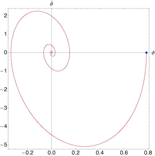
(The blue dot shows the chosen starting point of \( \dot{\phi} = 0, \phi = \pi/4 \); starting at the origin here wouldn't be very interesting.)
This diagram would look qualitatively the same, for essentially any choice of initial conditions that we took. Regardless of where the system starts, it will eventually spiral in to the same point \( (0,0) \) (ignoring oddball, unstable equilibria like \( \phi = \pi \).) Clearly there is something significant about \( (0,0) \) here, and in fact we say that the origin is an attractor; for a wide range of initial states, our system will always evolve in phase space towards the attractor.
Here, the attractor is an equilibrium point; all of the motion of the system dies down as we approach it. But an attractor can correspond to more interesting long-term behavior of the system. For example, if we now turn on the drive strength and set it to something weak, say \( \gamma = 0.2 \), then the phase-space orbit looks like this:
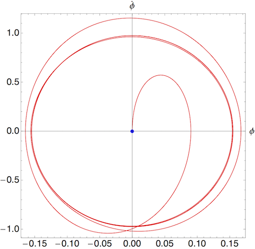
Due to the driving force, the pendulum is pushed away from the origin, eventually reaching a stable, essentially circular phase-space orbit. This orbit is another example of an attractor; even if we start the pendulum in some other initial state, it will wind up in exactly the same orbit if we wait long enough:

Here's the same plot starting at \( t=5 \), i.e. with the initial paths away from the starting points removed:
![]()
The initial part of the time evolution which depends on where we start the system is known as the transient part of the time evolution; with the transient behavior removed, we can see easily that all four starting points eventually settle into the same attractor state.
In general, we can classify attractors by their dimension. The origin with \( \gamma = 0 \) is a dimension-zero attractor, because it's just a point. The loop or limit cycle which appears with \( \gamma = 0.2 \) is said to be a dimension-one attractor, because the system moves along a (curled-up) line. Attractors of higher dimension can appear in more complicated systems; if we had a double pendulum with a four-dimensional phase space, we might find that it approached a dimension-two limit torus around which both angles \( \phi_1 \) and \( \phi_2 \) oscillated in some interdependent way.
We'll come back to the idea of attractors later, but for now let's just see what happens when we crank up the driving force. (As you can guess, there is chaotic motion in this system somewhere!)
The road to chaos
For a while, as we increase \( \gamma \) nothing much changes; we still find a limit cycle in the long-term behavior of the pendulum. However, at around \( \gamma \approx 1.07 \), something strange happens. If we plot the time series of \( \phi \) at \( \gamma = 1.073 \), this is what we see:
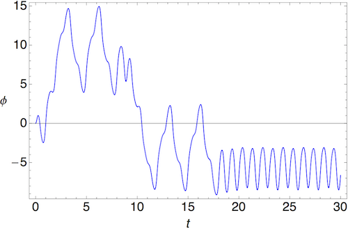
As we saw above, after some initial transient motion, the system settles down into a simple, periodic behavior. Except something doesn't look quite right about the oscillating behavior, if you look closely. In fact, if we zoom in, this is what we see:
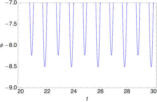
The peaks are at alternating heights! In fact, this system is no longer oscillating with period 1 (set by the drive frequency I picked above), but now it has twice the expected period. This phenomenon is known as period doubling. It is not chaotic motion; as you can see, the motion is still very predictable. But this period doubling is something which occurs when chaos is approached, in many systems, not just this one. If we plot the phase-space trajectory (after the transients have died down), we can see it's now following a limit cycle which looks like two joined loops:

There is a range of \( \gamma \) values around the one we picked which will exhibit the same period-two behavior; if we increase a bit further, we will observe another doubling, and the system will oscillate with period four. In fact, if we tune \( \gamma \) extremely carefully, we find transitions occuring at the following points:
| \( \gamma \) | period |
|---|---|
| 1.0663 | 1-->2 |
| 1.0793 | 2-->4 |
| 1.0821 | 4-->8 |
| 1.0827 | 8-->16 |
The distances in \( \gamma \) between period doublings diminishes quickly; in fact, it follows the formula
\[ \begin{aligned} \gamma_{n+1} - \gamma_n \approx \frac{1}{\delta} (\gamma_n - \gamma_{n-1}), \end{aligned} \]
where the constant \( \delta \approx 4.669 \) is a transcendental number (like \( e \) or \( \pi \)) known as the Feigenbaum number. This number is not special to the pendulum; period doubling following this exact formula appears in many other systems as they approach chaotic motion.
There is a neat way to visualize this repeated period doubling, by way of what is called a bifurcation diagram. We construct this diagram simply by taking samples of the function \( \phi(t) \) at regular intervals equal to the period for weak driving, after some initial wait for the transient signal to die off. By construction, at weak driving we sample once per period, so we get the same point back every time. However, once period doubling occurs, our set of sampled points will consist of two points, one from each of the sub-oscillations.
(You can imagine doing this experiment in a lab by taking a strobe light, and setting its frequency equal to the expected frequency of oscillation. For weak driving, the pendulum will appear frozen in one place; after one period doubling, you will see it in two places, then four, then eight, and so on.)
If we plot the results of this construction vs. \( \gamma \), with a timestep of \( \Delta t = 1 \) given our chosen driving frequency, we arrive at the bifurcation diagram, which shows a line that splits apart every time there is a period doubling:
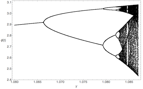
What's happening on the right side here? Well, since the distance between successive \( \gamma \)'s is decreasing quickly, the sequence of period doublings will eventually terminate - it will go to infinity at some finite critical value of the drive strength, which happens to be equal to
\[ \begin{aligned} \gamma_c = 1.0829. \end{aligned} \]
Beyond this value, we see chaotic motion for the first time! Setting \( \gamma = 1.105 \), we see a time-series that looks like this:

This is chaotic motion; it is aperiodic. No matter how long you wait, you will never find a regular repeating pattern in this time series, leading to the enormous scatter of points when we attempt to add it to the bifurcation diagram.
As we stressed at the beginning, one of the hallmarks of chaos is not just randomness, but sensitivity to initial conditions. Now we can see what that means quantitatively. At weak drive strength, because of the existence of attractors, we saw that starting with different initial conditions eventually leads us to indistinguishable motion. In terms of the time series, we see behavior that looks like this, taken at \( \gamma = 0.1 \):
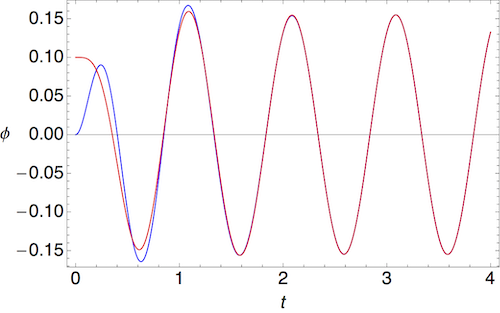
The two curves start at different values of \( \phi \), 0 and 0.1, but eventually converge and become indistinguishable. In fact, the convergence is quite rapid; if we plot the logarithm of the difference between the red and blue curves, this is what we find:
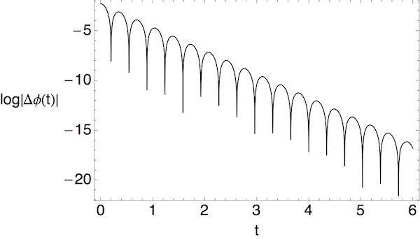
Up to some oscillations, the overall tendency is for this difference to exponentially vanish as the system evolves.
In the chaotic regime, on the other hand, we observe precisely the opposite behavior. At \( \gamma = 1.105 \) again, even starting now with an initial separation of \( 10^{-4} \), we find that the \( \phi(t) \) curves quickly separate:
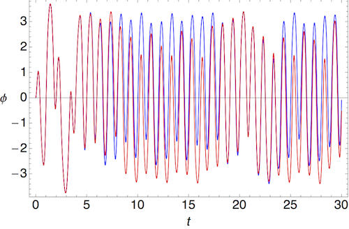

This time, the separation grows exponentially. In either case, we can model the behavior of the difference \( \Delta \phi \) as
\[ \begin{aligned} |\Delta \phi(t)| \sim K e^{\lambda t}. \end{aligned} \]
The coefficient in the exponent \( \lambda \), which is the slope of the linear trend on these log plots, is known as the Liapunov exponent, and it is negative for periodic systems which approach an attractor, and positive for chaotic systems.
We should note at this point that initial condition sensitivity is necessary for chaos, but it's not sufficient. The simple mathematical function \( f(x) = c 2^x \) has extreme sensitivity to the value of \( c \), and for different \( c \) the functions will diverge exponentially from each other. But it isn't an example of chaotic motion. A rigorous mathematical definition of chaos is beyond us in this course, but suffice it to say that chaos requires that the motion be complicated and dense (in the mathematical sense.) Here's the phase-space evolution of a chaotic pendulum, now at the slightly smaller but still chaotic value \( \gamma = 1.086 \):
(Once again the initial transient motion has been removed here.) You can see what I mean by "dense" here!
The density of the curves makes it a little hard to see exactly what's going on in phase space for the chaotic pendulum, although you can certainly tell that there's some structure to the time evolution, despite the chaotic behavior. You could also guess this from the bifurcation diagram; even in the chaotic region, there is some structure to how the observations for \( \phi(t) \) after each timestep are distributed.
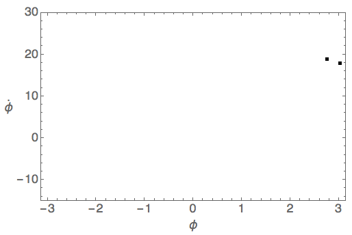
One more useful way to plot this system is using something called a Poincaré section. This is, essentially, a combination of a phase-space plot and a bifurcation diagram: we again sample at the weak driving period (\( \Delta t = 1 \) here), but we take both \( \phi(t) \) and \( \phi'(t) \) and plot the results of our sampling in phase space. For simple periodic motion, say at \( \gamma = 1.065 \), this gives us a single point:

because every time we move by 1 period, the system is in exactly the same state. (This plot is actually 600 points, but they're all stacked on top of each other.) You can probably guess that when we hit the period-doubling transition, we will see two points instead of one, reflecting the doubled period:
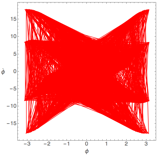
Very simple, so far! But when we push the drive strength into the chaotic region, the plot becomes really remarkable:

(Here I've reduced the damping to \( \beta = \omega_0 / 8 \) and taken \( \gamma = 1.5 \), following Taylor.) Zooming in on one of the "tongue" regions in the plot reveals deeper structure:
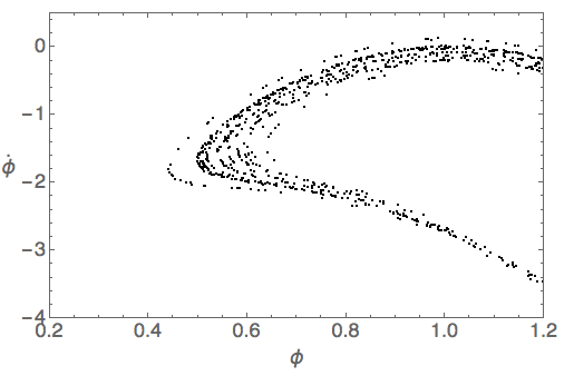
If I ran with more points, we could keep zooming in and would find similar structures further and further down. This is an example of fractal geometry; finding similar structures after zooming in is a characteristic feature of such objects.
This takes me back to one last parting comment on classical chaos. This Poincaré section reveals that even chaotic systems can exhibit attractor behavior, but the curve they approach is known as a strange attractor. If we try to calculate the dimension of such an attractors, we inevitably find that it is non-integer; i.e., they have fractal dimension. The mathematics of fractals and chaos are closely intertwined, and quite beautiful, but that's a topic for another class.