Example: inertia tensor of a cube
Consider a cube of fixed density \( \rho \), side length \( b \), rotating about one of its corners. What is the inertia tensor?
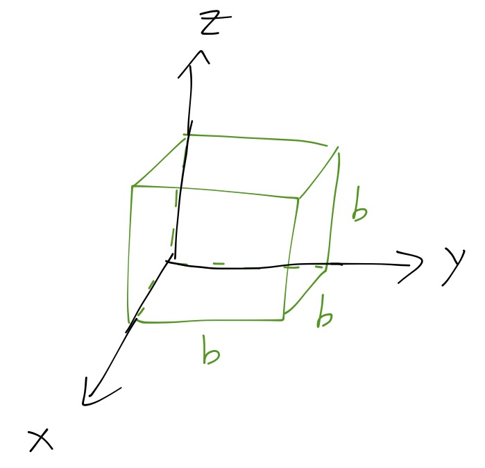
Before we begin, let's think about whether we really need to evaluate all six integrals in this case. The cube has a lot of symmetry; in particular, we can see immediately that it looks exactly the same in the \( x \), \( y \), and \( z \) directions from our starting point. So exchanging the variables \( x,y,z \) will give us the same integral and thus the same answer. This tells us that the three off-diagonal components of \( \mathbf{I} \) are all equal, and so are the three diagonal components.
There's no way to reduce further; the diagonal and off-diagonal integrals look different, and none of them are obviously equal to zero. So we have 2 integrals to evaluate.
Let's start with the top left diagonal component. Since \( \rho \) is constant, we can pull it out of integral:
\[ \begin{aligned} I_{xx} = \rho \int_0^b dx \int_0^b dy \int_0^b dz (y^2 + z^2) \\ = b \rho \int_0^b dy \left.(y^2 + \frac{1}{3} z^3)\right|_0^b \\ = b \rho \int_0^b dy (by^2 + \frac{1}{3} b^3) \\ = b \rho (\frac{1}{3} b^4 + \frac{1}{3} b^4) = \frac{2}{3} \rho b^5 = \frac{2}{3} Mb^2. \end{aligned} \]
where at the last step I've identified that the density of the cube can be rewritten as \( M = \rho b^3 \). Now, the off-diagonal component:
\[ \begin{aligned} I_{xy} = \rho \int_0^b dx \int_0^b dy \int_0^b dz (-xy) \\ = -b \rho \int_0^b dx (\frac{1}{2} x b^2) \\ = -\frac{1}{4} \rho b^5 = -\frac{1}{4} Mb^2. \end{aligned} \]
All off-diagonal components are the same, and all diagonal components too, thanks to the symmetry of the cube! So the full tensor is:
\[ \begin{aligned} \overset\leftrightarrow I = Mb^2 \left( \begin{array}{ccc} \frac{2}{3} & -\frac{1}{4} & -\frac{1}{4} \\ -\frac{1}{4} & \frac{2}{3} & -\frac{1}{4} \\ -\frac{1}{4} & -\frac{1}{4} & \frac{2}{3} \end{array} \right). \end{aligned} \]
As we've just seen, it's very helpful to identify the symmetries of our object before we start calculating integrals! Often you'll be able to demonstrate using symmetry either that some components of the inertia tensor are equal to each other, or even that they must be zero (for the off-diagonal components.)
Once again, I'll stress that the location of the pivot point is important! You know from intro physics that a cylinder has a different moment of inertia for rotation about its edge or about its center, for example. In our cube example above, we can only use the expression we found for rotations that pass through the corner of the cube; for other pivot points, \( \mathbf{I} \) will change!
Let's see explicitly what the difference is, by recomputing the cube's inertia tensor from its center of mass.
Example: inertia tensor of a cube about the CM
Much like the cube about its corner, the high degree of symmetry here means we only need to do two out of nine possible integrals. Let's look at a diagonal element first:
\[ \begin{aligned} I_{xx} = \int\ dV \rho (y^2 + z^2) \\ = \rho \int_{-b/2}^{b/2} dx \int_{-b/2}^{b/2} dy \int_{-b/2}^{b/2} dz (y^2 + z^2) \\ = \rho b \int_{-b/2}^{b/2} dy \left. (zy^2 + \frac{1}{3} z^3) \right|_{-b/2}^{b/2} \\ = \rho b \int_{-b/2}^{b/2} dy \left( by^2 + \frac{1}{3} \frac{b^3}{4} \right) \\ = \rho b \left. \left( \frac{1}{3} by^3 + \frac{1}{12} b^3 y \right) \right|_{-b/2}^{b/2} \\ = \rho b \left( \frac{1}{12} b^4 + \frac{1}{12} b^4 \right) \\ = \frac{1}{6} \rho b^5 = \frac{1}{6} M b^2. \end{aligned} \]
On the other hand, all the off-diagonal moments are zero, for example
\[ \begin{aligned} I_{xy} = \int\ dV \rho (-xy). \end{aligned} \]
This is an odd function of \( x \) and \( y \), and our integration is now symmetric about the origin in all directions, so it vanishes identically. So the inertia tensor of the cube about its center is
\[ \begin{aligned} \mathbf{I} = \frac{1}{6} Mb^2 \left( \begin{array}{ccc} 1 & 0 & 0 \\ 0 & 1 & 0 \\ 0 & 0 & 1 \end{array} \right). \end{aligned} \]
Example: principal axes for a cube rotating about a corner
Now let's have a look at finding the principal moments and principal axes. We'll go back to the cube rotating about its corner for this, which we found to have inertia tensor equal to
\[ \begin{aligned} \overset\leftrightarrow I = Mb^2 \left( \begin{array}{ccc} \frac{2}{3} & -\frac{1}{4} & -\frac{1}{4} \\ -\frac{1}{4} & \frac{2}{3} & -\frac{1}{4} \\ -\frac{1}{4} & -\frac{1}{4} & \frac{2}{3} \end{array} \right) = \mu \left(\begin{array}{ccc} 8 & -3 & -3 \\ -3 & 8 & -3 \\ -3 & -3 & 8 \end{array} \right) \end{aligned} \]
where I've introduced \( \mu \equiv Mb^2 / 12 \) to save some space. To find the principal axes, we must start by finding the eigenvalues of this matrix, which are solutions to the characteristic equation
\[ \begin{aligned} \det(\mathbf{I} - \lambda \mathbf{1}) = 0. \end{aligned} \]
where \( \mathbf{1} \) is the identity matrix (to avoid using the notation \( I \) twice.) In other words,
\[ \begin{aligned} \left| \begin{array}{ccc} 8\mu - \lambda & -3\mu & -3\mu \\ -3\mu & 8\mu - \lambda & -3\mu \\ -3\mu & -3\mu & 8\mu - \lambda \end{array} \right| = 0. \end{aligned} \]
The book says this determinant is "straightforward to evaluate"; that only happens to be true if you think solving cubic equations by hand is straightforward. I'll show you a way to do this in the online lecture notes, and of course Mathematica can do it, but here we'll skip to the results.
(Here follows the solution that we skipped in class for the characteristic polynomial; it's not a foolproof way to solve cubics, but it shows a nice way to guess at such a solution.)
Expanding in minors
$$ \begin{aligned} (8\mu - \lambda) [(8\mu - \lambda)^2 - 9\mu^2] + 3\mu \
- 3\mu [9\mu^2 + 3\mu (8\mu - \lambda)] = 0
\end{aligned} $$
Gathering terms,
\[ \begin{aligned} (8\mu - \lambda)^3 - 27\mu^2 (8\mu - \lambda) - 54 \mu^3 = 0 \\ (512 - 216 - 54) \mu^3 + 24 \mu \lambda^2 + (192-27) \mu^2 \lambda - \lambda^3 = 0 \\ 242 \mu^3 + 24 \mu \lambda^2 - 165 \mu^2 \lambda - \lambda^3 = 0. \end{aligned} \]
where as you will remember, \( (x+y)^3 = x^3 + 3x^2 y + 3xy^2 + y^3 \). We can factorize this by assuming the form \( (a-\lambda)(b-\lambda)(c-\lambda) \), which expands out to
$$ \begin{aligned} (a-\lambda)(bc - \lambda (b+c) + \lambda^2) = abc - a(b+c) \lambda \
- a\lambda^2 -bc \lambda + \lambda^2 (b+c) - \lambda^3
= -\lambda^3 + \lambda^2 (a+b+c) - \lambda (ab + ac + bc) + abc. \end{aligned} $$
so for our determinant,
\[ \begin{aligned} a+b+c = 24\mu \\ ab + ac + bc = 165\mu^2 \\ abc = 242 \mu^3. \end{aligned} \]
There's not a really nice way to solve these equations in general, but we can notice from the last equation that the prime factors of 242 are 2, 11, and 11. If you try those values for a, b, c, you will see that they do in fact work: their sum is 24, and the sum of products in the middle is \( 22 + 22 + 121 = 165 \).
Whether we solve by hand or not, we will arrive at the factorized characteristic polynomial:
\[ \begin{aligned} (2\mu - \lambda) (11\mu - \lambda)^2 = 0. \end{aligned} \]
The eigenvalues are thus \( \lambda_1 = 2\mu \) and \( \lambda_2 = \lambda_3 = 11\mu \). To find the eigenvectors, we go back to the eigenvalue equation and plug in each eigenvalue one by one. First,
\[ \begin{aligned} (\mathbf{I} - \lambda_1 \mathbf{1}) \vec{v}_1 = \mu \left( \begin{array}{ccc} 6&-3&-3 \\ -3&6&-3 \\ -3&-3&6 \end{array} \right) \left( \begin{array}{c} v_{1,x} \\ v_{1,y} \\ v_{1,z} \end{array} \right) = 0. \end{aligned} \]
In lecture, I used row reduction to manipulate these equations: here I'll do the same thing by expanding out in components.
\[ \begin{aligned} 2 v_{1,x} - v_{1,y} - v_{1,z} = 0 \\ -v_{1,x} + 2v_{1,y} - v_{1,z} = 0 \\ -v_{1,x} - v_{1,y} + 2v_{1,z} = 0. \end{aligned} \]
The first two equations combine to give us
\[ \begin{aligned} 3v_{1,x} - 3v_{1,y} = 0, \end{aligned} \]
so \( v_{1,x} = v_{1,y} \), and then from the final equation
\[ \begin{aligned} -2v_{1,x} + 2v_{1,z} = 0 \end{aligned} \]
so \( v_{1,x} = v_{1,z} \) as well. Thus, the first eigenvector points in the direction \( (1,1,1) \); rescaling to a unit vector, we have
\[ \begin{aligned} \hat{e}_1 = \frac{1}{\sqrt{3}} (1,1,1). \end{aligned} \]
So the principal axis corresponding to the smallest eigenvalue \( \lambda = 2\mu \) points along the diagonal of the cube. Notice that we didn't need the third equation; if we were doing row reduction, we would have found one row reduces to \( (0,0,0) \). This is completely as expected! Eigenvectors are only unique up to a constant - their length is undetermined - so we should only have two unique equations in three unknowns.
Doing the same thing for the next eigenvalue, we find the matrix equation:
\[ \begin{aligned} (\mathbf{I} - \lambda_1 \mathbf{1}) \vec{v}_2 = \mu \left( \begin{array}{ccc} -3&-3&-3 \\ -3&-3&-3 \\ -3&-3&-3 \end{array} \right) \left( \begin{array}{c} v_{2,x} \\ v_{2,y} \\ v_{2,z} \end{array} \right) = 0. \end{aligned} \]
Now we have two redundant equations; the one remaining equation can be rewritten in the form
\[ \begin{aligned} \vec{v}_2 \cdot (1,1,1) = 0, \end{aligned} \]
But this is just the vector geometric statement that \( \vec{v}_2 \) lies anywhere in the plane perpendicular to the first eigenvector, \( (1,1,1) \). Moreover, \( \vec{v}_3 \) gives exactly the same equation, since it has the same principal moment. (This is an example of a degeneracy, which is when two eigenvalues of a matrix are equal.)
Although \( \vec{v}_2 \) and \( \vec{v}_3 \) aren't uniquely determined, they must both be orthogonal to \( \vec{v}_1 \), and they must be orthogonal to each other. Thus, we may choose any pair of vectors satisfying these conditions, for example
\[ \begin{aligned} \hat{e}_2 = \frac{1}{\sqrt{6}} (2,-1,-1) \\ \hat{e}_3 = \frac{1}{\sqrt{2}} (0,1,-1). \end{aligned} \]
Any combination of these vectors is also an eigenvector, so this is not a unique choice; physically, this means that it doesn't matter how we rotate \( \hat{e}_2 \) and \( \hat{e}_3 \) with each other, our inertia tensor remains diagonal.
With our choice of coordinates complete, the inertia tensor in these (body-frame) coordinates provided by the eigenvectors is now diagonal:
\[ \begin{aligned} \mathbf{I} = \frac{1}{12} Mb^2 \left( \begin{array}{ccc} 2 & 0 & 0 \\ 0 & 11 & 0 \\ 0 & 0 & 11 \end{array} \right). \end{aligned} \]
You can think of the cube as standing on its point in these coordinates, with the \( \hat{e}_1 \) axis pointing through the diagonal of the cube vertically.