Example: springs on a ring
Here's another example which will show some unique features that appear in certain versions of the coupled oscillator problem. We consider three identical masses \( m \) arranged on a ring, and connected by three identical springs with force constant \( k \):

The kinetic energy is easy here:
\[ \begin{aligned} T = \frac{1}{2} mR^2 (\dot{\phi}_1^2 + \dot{\phi}_2^2 + \dot{\phi}_3^2) \end{aligned} \]
As for the potential, the length of the arc between any two springs is \( R (\phi_i - \phi_j) \). Angles are a little tricky, though, since there are factors of \( 2\pi \) floating around: if \( \phi_1 = 0.1 \) and \( \phi_3 = 2\pi - 0.1 \), for example, they're actually fairly close together. It's better to use displacements from equilibrium as usual:
\[ \begin{aligned} \beta_1 = \phi_1 \\ \beta_2 = \phi_2 - 2\pi / 3 \\ \beta_3 = \phi_3 - 4\pi / 3 \end{aligned} \]
Mathematically we should restrict what values these things can take on, but we know physically the springs will prevent anything too strange (e.g. the masses passing through each other) from happening, so we'll just go ahead and solve in these coordinates. The potential is
\[ \begin{aligned} U = \frac{1}{2} kR^2 \left( (\beta_2 - \beta_1)^2 + (\beta_3 - \beta_2)^2 + (\beta_1 - \beta_3)^2 \right) \end{aligned} \]
We have three equations of motion to find. Let's start with \( \beta_1 \):
\[ \begin{aligned} \frac{\partial \mathcal{L}}{\partial \beta_1} = \frac{d}{dt} \left( \frac{\partial \mathcal{L}}{\partial \dot{\beta}_1} \right) \\ -kR^2 (2\beta_1 - \beta_2 - \beta_3) = m R^2 \ddot{\beta}_1. \end{aligned} \]
Since the Lagrangian is totally symmetric between the three \( \beta_i \), it's easy to see that the other two equations look more or less the same, i.e.
\[ \begin{aligned} -k (-\beta_1 + 2\beta_2 - \beta_3) = m \ddot{\beta}_2 \\ -k (-\beta_1 - \beta_2 + 2\beta_3) = m \ddot{\beta}_3. \end{aligned} \]
where all the \( R^2 \) factors cancel out. From here, we read off the two matrices.
\[ \begin{aligned} \mathbf{K} = \left( \begin{array}{ccc} 2k & -k & -k \\ -k & 2k & -k \\ -k & -k & 2k \end{array} \right) \end{aligned} \]
and
\[ \begin{aligned} \mathbf{M} = \left( \begin{array}{ccc} m & 0 & 0 \\ 0 & m & 0 \\ 0 & 0 & m \end{array} \right), \end{aligned} \]
so our eigenvalue equation is
\[ \begin{aligned} \left| \begin{array}{ccc} 2k-\omega^2 m & -k & -k \\ -k & 2k - \omega^2 m & -k \\ -k & -k & 2k - \omega^2 m \end{array} \right| = 0. \end{aligned} \]
I won't go through the gory details on the board, but the result of this determinant is
\[ \begin{aligned} m^3 \omega^2 \left(\omega^4 - 6(k/m) \omega^2 + 9(k/m)^2 \right) = 0. \end{aligned} \]
The cubic nicely factorizes for us, so one eigenvalue is just \( \omega_1 = 0 \). For the other two, we solve the quadratic:
\[ \begin{aligned} \omega^2 = \frac{1}{2} \left[ \frac{6k}{m} \pm \sqrt{\frac{36k^2}{m^2} - 4 \frac{9k^2}{m^2}} \right] \\ = \frac{3k}{m}. \end{aligned} \]
Yes, only one solution, so \( \omega_2^2 = \omega_3^2 = 3k/m \).
Now, what are the normal modes for each of these frequencies? We'll start with \( \omega_1 = 0 \): plugging back into the eigenvalue problem matrix,
\[ \begin{aligned} \left( \begin{array}{ccc} 2k & -k & -k \\ -k & 2k & -k \\ -k & -k & 2k \end{array} \right) \left( \begin{array}{c} \xi_x \\ \xi_y \\ \xi_z \end{array} \right) = 0 \end{aligned} \]
This is straightforward to row-reduce, but you may also be able to spot immediately that the vector which solves all three equations is simply
\[ \begin{aligned} \vec{\xi}_1 = \left( \begin{array}{c} 1 \\ 1 \\ 1 \end{array} \right). \end{aligned} \]
This corresponds to equal displacement of all three masses in the same direction. But this can't be a normal periodic motion, because the frequency is zero. If we remember that we're solving for the acceleration, then zero frequency is just the differential equation \( \ddot{\vec{x}} = 0 \), i.e. movement with constant velocity.
Physically, we see that this is totally reasonable: if all three masses move with constant speed around the ring in the same direction, then the springs are never stretched, and there are no forces! This sort of motion is known as a zero mode of the system, since it corresponds to a solution to the coupled oscillator equation with \( \omega = 0 \). For example, in the motion of two blocks coupled by a single spring (and with no other forces), the motion of the center of mass of the two blocks is a zero mode.

Now, what about the other normal modes? Since we have degenerate eigenvalues, we expect some ambiguity in finding them. The eigenvector equation with \( \omega^2 = 3k/m \) is
\[ \begin{aligned} \left( \begin{array}{ccc} -k & -k & -k \\ -k & -k & -k \\ -k & -k & -k \end{array} \right) \left( \begin{array}{c} \xi_x \\ \xi_y \\ \xi_z \end{array} \right) = 0 \end{aligned} \]
No row reduction necessary! This is the same equation repeated three times, namely
\[ \begin{aligned} \xi_x + \xi_y + \xi_z = 0, \end{aligned} \]
which is (of course) just the condition that these other normal modes are both orthogonal to the first one we found (the zero mode.) As always in this situation, we're free to pick any two orthogonal vectors that satisfy this condition, let's say
\[ \begin{aligned} \vec{\xi}_2 = \left( \begin{array}{c} 1 \\ -1 \\ 0 \end{array} \right) \\ \vec{\xi}_3 = \left( \begin{array}{c} 1 \\ 0 \\ -1 \end{array} \right) \end{aligned} \]
So the second mode corresponds to masses 1 and 2 oscillating back and forth, while mass 3 is stationary:
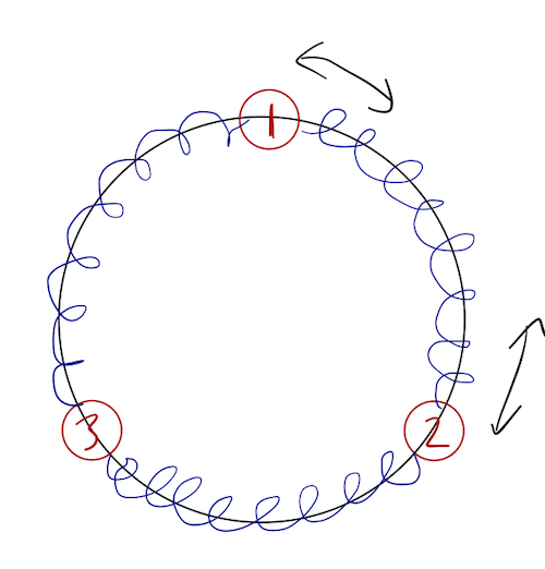
The third mode is the same thing, but with masses 1 and 3 oscillating and mass 2 fixed.
Of course, this problem is very symmetric, so we should ask: what about the possibility of mass 1 being fixed while 2 and 3 oscillating? That "direction" is just a difference of the other two modes, i.e.
\[ \begin{aligned} \vec{\xi}_2 - \vec{\xi}_3 = \left( \begin{array}{c} 0 \\ -1 \\ 1 \end{array} \right). \end{aligned} \]
Ordinarily this would be a combination of two different oscillations, but because \( \vec{\xi}_2 \) and \( \vec{\xi}_3 \) have the same normal frequency, this combination is also simply a normal mode. It's easier to see what's happening if we write the general solution out:
\[ \begin{aligned} \vec{\phi}(t) = A_0 + B_0 t + A_1 \left( \begin{array}{c} 1 \\ -1 \\ 0 \end{array} \right) \cos (\sqrt{3k/m} t + \delta_1) + A_2 \left( \begin{array}{c} 1 \\ 0 \\ -1 \end{array} \right) \cos (\sqrt{3k/m} t + \delta_2) \end{aligned} \]
Since the latter two terms have the same frequency, we can combine them and end up with an oscillation proportional to another vector, just with a different amplitude and phase. The only restriction is that the resulting vector always satisfies \( \xi_x + \xi_y + \xi_z = 0 \).
In the end, the motion of this system isn't too interesting: all possible motions of the springs are combinations of zero-mode motion, and some oscillation at the fixed frequency \( \omega = \sqrt{3k/m} \), such that the positions of the three masses always satisfy \( \beta_1 + \beta_2 + \beta_3 = 0 \). If we changed one of the masses or spring constants, in general we'd find three distinct normal modes and more complicated motion. (The zero-mode will always remain, no matter what.)
Example: the double pendulum
For the most part, there's not too much difficulty in expanding the framework we've needed to bigger and more complex systems. Certainly a big collection of carts and springs won't make things more interesting; it will just force us to deal with bigger matrices. But it's worth looking at some coupled oscillators that aren't just springs and masses, to illustrate some more general features. So let's consider the double pendulum:
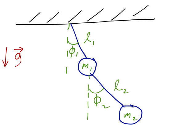
We've thought about setting up the Lagrangian for this system before. Starting with the potential energy, for mass 1 we simply have
\[ \begin{aligned} U_1 = m_1 g \ell_1 (1 - \cos \phi_1) \end{aligned} \]
doing a bit of geometry and checking that the potential is smallest (zero, in these coordinates) at \( \phi_1 = 0 \). The potential energy of mass 2 is similar, except that we have to add the vertical position of the first mass as well:
\[ \begin{aligned} U_2 = m_2 g [\ell_1 (1 - \cos \phi_1) + \ell_2 (1 - \cos \phi_2)]. \end{aligned} \]
As for the kinetic energy, we can think of it in terms of vectors. Because mass 1 only moves by changing \( \phi_1 \), its velocity vector points in the \( \hat{\phi}_1 \) direction:
\[ \begin{aligned} \vec{v}_1 = \ell_1 \dot{\phi}_1 \hat{\phi}_1 \end{aligned} \]
so
\[ \begin{aligned} T_1 = \frac{1}{2} m_1 v_1^2 = \frac{1}{2} m_1 \ell_1^2 \dot{\phi}_1^2. \end{aligned} \]
Of course, I didn't need to write this as a vector; we know that this is what the kinetic energy of rotation about a point at fixed distance \( \ell_1 \) looks like. But mass 2 has a more complicated kinetic term; its position depends on the position of mass 1 as well.
Since we've set this up in terms of velocity vectors, all we need to do is square our expression for \( \vec{v}_2 \), which is
\[ \begin{aligned} \vec{v}_2 = \ell_1 \dot{\phi}_1 \hat{\phi}_1 + \ell_2 \dot{\phi}_2 \hat{\phi}_2 \end{aligned} \]
Then
\[ \begin{aligned} |\vec{v}_2|^2 = \vec{v}_2 \cdot \vec{v}_2 = \ell_1^2 \dot{\phi}_1^2 + \ell_2^2 \dot{\phi}_2^2 + 2 \ell_1 \ell_2 \dot{\phi}_1 \dot{\phi}_2 (\hat{\phi}_1 \cdot \hat{\phi}_2). \end{aligned} \]
The dot product of the two unit vectors is equal to the cosine of the angle between them, which is \( (\phi_2 - \phi_1) \).
At this point, I'm going to set \( m_1 = m_2 = m \) and \( \ell_1 = \ell_2 = \ell \), just to make things simpler to work through. Doing so, our total Lagrangian for this system from the pieces we have found is
\[ \begin{aligned} \mathcal{L} = m \ell^2 \dot{\phi}_1^2 + \frac{1}{2} m \ell^2 \dot{\phi}_2^2 + m \ell^2 \dot{\phi}_1 \dot{\phi}_2 \cos(\phi_1 - \phi_2) \\ \ + mg \ell \left( 2\cos \phi_1 + \cos \phi_2 \right) \end{aligned} \]
We can go on to write the equations of motion, but it's clear we won't be able to write it in the linear form that we used to solve the coupled mass and spring system, because of the cosines. But we know how to deal with the cosines already, from studying a single pendulum: we make a small-angle approximation. We'll keep terms up to order \( \phi^2 \) or \( \dot{\phi}^2 \) in the Lagrangian, to end up with terms of order \( \phi \) after taking derivatives to find the equations of motion. Thus, using
\[ \begin{aligned} \cos(x) \approx 1 - \frac{x^2}{2}, \end{aligned} \]
we find the approximate result
\[ \begin{aligned} \mathcal{L} \approx m\ell^2 \dot{\phi}_1^2 + \frac{1}{2} m\ell^2 \dot{\phi}_2^2 + m \ell^2 \dot{\phi}_1 \dot{\phi}_2 - \frac{1}{2} mg \ell (2 \phi_1^2 + \phi_2^2). \end{aligned} \]
Now we can differentiate:
\[ \begin{aligned} \frac{\partial \mathcal{L}}{\partial \phi_1} = \frac{d}{dt} \frac{\partial \mathcal{L}}{\partial \dot{\phi}_1} \\ -2mg\ell \phi_1 = 2m\ell^2 \ddot{\phi}_1 + m\ell^2 \ddot{\phi}_2 \\ -mg\ell \phi_2 = m\ell^2 \ddot{\phi}_2 + m\ell^2 \ddot{\phi}_1. \end{aligned} \]
We can write this in the usual matrix form, \( \mathbf{M} \ddot{\vec{\phi}} = -\mathbf{K} \vec{\phi} \), except now \( M \) is the more complicated matrix:
\[ \begin{aligned} \mathbf{M} = m\ell^2 \left( \begin{array}{cc} 2 & 1 \\ 1 & 1 \end{array} \right) \\ \mathbf{K} = -m\ell^2 \left( \begin{array}{cc} 2\omega_0^2 & 0 \\ 0 & \omega_0^2 \end{array} \right) \end{aligned} \]
where for convenience, I've defined the constant \( \omega_0 = \sqrt{g/\ell} \), which you'll recognize as the usual frequency for small oscillations of a pendulum. Cancelling the common factor of \( m\ell^2 \), we can then write the combined matrix for the generalized eigenvalue problem as
\[ \begin{aligned} \mathbf{K} - \omega^2 \mathbf{M} = \left( \begin{array}{cc} 2 (\omega_0^2 - \omega^2) & -\omega^2 \\ -\omega^2 & (\omega_0^2 - \omega^2) \end{array} \right) \end{aligned} \]
which has determinant
\[ \begin{aligned} \det(\mathbf{K} - \omega^2 \mathbf{M}) = 2(\omega_0^2 - \omega^2)^2 - \omega^4 = 0 \\ \omega^4 - 4 \omega_0^2 \omega^2 + 2\omega_0^2 = 0. \end{aligned} \]
This is just a simple quadratic equation, and the roots are
\[ \begin{aligned} \omega^2 = \omega_0^2 (2 \pm \sqrt{2}). \end{aligned} \]
As always, we plug back in to find the eigenvectors; I'll skip the details, but you can verify that the result we get is
\[ \begin{aligned} \omega_1^2 = \omega_0^2 (2 - \sqrt{2}), \hat{\xi}_1 = \frac{1}{\sqrt{3}}\left(\begin{array}{c} 1 \\ \sqrt{2} \end{array} \right) \\ \omega_2^2 = \omega_0^2 (2 + \sqrt{2}), \hat{\xi}_2 = \frac{1}{\sqrt{3}} \left(\begin{array}{c} 1 \\ -\sqrt{2} \end{array} \right). \end{aligned} \]
and as usual, the general solution is given by combining the two,
\[ \begin{aligned} \vec{\phi}(t) = A_1 \hat{\xi}_1 \cos (\omega_1 t - \delta_1) + A_2 \hat{\xi}_2 \cos (\omega_2 t - \delta_2) \\ = \left(\begin{array}{c} A_1 \cos (\omega_1 t - \delta_1) + A_2 \cos(\omega_2 t - \delta_2) \\ \sqrt{2} A_1 \cos (\omega_1 t - \delta_1) - \sqrt{2} A_2 \cos (\omega_2 t - \delta_2) \end{array} \right). \end{aligned} \]
What does motion in each of the normal modes look like? For the first mode (\( A_2 = 0 \)), the two masses oscillate completely in phase, but the amplitude (in \( \phi_2 \)) of the lower component is larger by a factor of \( \sqrt{2} \) (so it will swing out further.) In the second mode, the amplitudes are the same, but the motion is \( 180^{\circ} \) out of phase; they swing in opposite directions.
Example: Vibrational energy of carbon dioxide
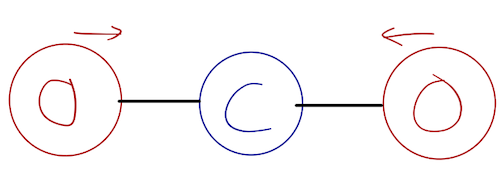
Here's a system that you probably didn't think you'd see in classical mechanics: a carbon dioxide molecule.

CO2 is a nice molecule to deal with, because the atoms are arranged more or less in a straight line. Molecules can exist in what are called excited states, where they have extra energy stored inside them; vibrational motion is one example of how this energy can be stored.
There are a few different ways that a CO2 molecule can vibrate, but let's focus on just one-dimensional motion in the direction along the molecule. Let's take \( m_O \) to be the mass of oxygen, and \( m_C \) the mass of carbon. In terms of the coordinates shown, we know that
\[ \begin{aligned} \mathcal{L} = \frac{1}{2} m_O\dot{x_1}^2 + \frac{1}{2} m_C\dot{x_2}^2 + \frac{1}{2} m_O\dot{x_3}^2 - V(x_1 - x_2) - V(x_2 - x_3). \end{aligned} \]
The potential \( V(r) \) corresponds to the interatomic binding energy, and in general is quite complicated. But we don't need to know its form to study small vibrations! The equilibrium point, given by the minimum-energy state, we take to be \( |x_1 - x_2| = r_0 \). By symmetry, \( |x_2 - x_3| = r_0 \) at equilibrium as well. As above, we expand in small displacements \( \eta \):
\[ \begin{aligned} x_i(t) = x_i^0 + \eta_i(t) \end{aligned} \]
By doing so, we can Taylor expand the unknown potential energy functions:
\[ \begin{aligned} V(r) = V(r_0) + \left. \frac{\partial V}{\partial r}\right|_{r=r_0} (r-r_0) + \frac{1}{2} \left.\frac{\partial^2 V}{\partial r^2} \right|_{r=r_0} (r-r_0^2) + ... \end{aligned} \]
The first term is just a constant, which we can drop. Because \( r=r_0 \) is an equilibrium point, we know that \( \partial V / \partial r \) must vanish there (think back to central-force motion; stable equilibrium with no evolution happens when \( E = V \) at a minimum of the potential.) We have no idea what the second derivative is, but at \( r=r_0 \) it is just a constant, which we'll call \( k \):
\[ \begin{aligned} \left.\frac{\partial^2 V}{\partial r^2}\right|_{r=r_0} \equiv k. \end{aligned} \]
With that, we can substitute back in to find the potential energies in terms of the \( \eta \)'s:
\[ \begin{aligned} V(x_1 - x_2) \approx \frac{k}{2} (x_1 - x_2 - r_0)^2 = \frac{k}{2} (\eta_1 - \eta_2)^2 \\ V(x_2 - x_3) \approx \frac{k}{2} (\eta_2 - \eta_3)^2 \end{aligned} \]
so the Lagrangian for the \( \eta \)'s is
\[ \begin{aligned} \mathcal{L} \approx \frac{1}{2} m_O (\dot{\eta_1}^2 + \dot{\eta_3}^2) + \frac{1}{2} m_C \dot{\eta_2}^2 - \frac{k}{2} \left[ (\eta_1 - \eta_2)^2 + (\eta_2 - \eta_3)^2 \right]. \end{aligned} \]
Taking the appropriate derivatives, the Euler-Lagrange equations of motion are then
\[ \begin{aligned} m_O \ddot{\eta_1} = -k(\eta_1 - \eta_2) \\ m_C \ddot{\eta_2} = -k(\eta_2 - \eta_1) - k (\eta_2 - \eta_3) \\ m_O \ddot{\eta_3} = -k(\eta_3 - \eta_2). \end{aligned} \]
Dividing through by the masses and rewriting as a matrix, we have
\[ \begin{aligned} \ddot{\vec{\eta}} = -\mathbf{F} \vec{\eta} \end{aligned} \]
where
\[ \begin{aligned} \mathbf{F} = \left( \begin{array}{ccc} k/m_O & -k/m_O & 0 \\ -k/m_C & 2k/m_C & -k/m_C \\ 0 & -k/m_O & k/m_O \end{array} \right) \end{aligned} \]
(Notice, by the way, that \( F \) is not a symmetric matrix! Still, all the eigenvalues will be real; this is guaranteed by the fact that the individual matrices \( M \) and \( K \) arising from the kinetic and potential energy are symmetric.)
As always, to solve for the motion, we find the eigenvalues and eigenvectors of this matrix. Defining \( (k/m_O) \lambda^2 = \omega^2 \) and \( \rho \equiv m_O/m_C \), the matrix we need for the eigenvalue problem is
\[ \begin{aligned} \mathbf{F} - \omega^2 \mathbf{I} = \frac{k}{m_O} \left( \begin{array}{ccc} 1-\lambda^2 & -1 & 0 \\ -\rho & 2\rho - \lambda^2 & -\rho \\ 0 & -1 & 1-\lambda^2 \end{array} \right) \end{aligned} \]
The characteristic equation is
\[ \begin{aligned} \det(\mathbf{F} - \omega^2 \mathbf{I}) = -(1-\lambda^2) [(2\rho - \lambda^2) (1-\lambda^2) - \rho] - \rho (1-\lambda^2) \\ = -(1-\lambda^2) \left [ \lambda^4 - (1 + 2\rho) \lambda^2 \right]. \end{aligned} \]
We can just read off the eigenvalues, since this is already nicely factorized:
\[ \begin{aligned} \omega_1 = \sqrt{k/m_O} \lambda_1 = 0 \\ \omega_2 = \sqrt{k/m_O} \lambda_2 = \sqrt{k/m_O} \\ \omega_3 = \sqrt{k/m_O} \lambda_3 = \sqrt{k/m_O (1 + 2m_O/m_C)}. \end{aligned} \]
If we solve for the eigenvectors, we find the range of motion we would expect: the first eigenvector is \( \vec{\xi}_1 = (1,1,1) \), corresponding to translation in space; there is no vibration at all, which we identify as a zero mode since \( \omega_1 = 0 \). The second and third modes are \( \vec{\xi}_2 = (1,0,-1) \) and \( \vec{\xi}_3 = (1,-2m_O/m_C, 1) \), corresponding to vibration of the oxygen atoms with C fixed (the symmetric stretch mode), and motion where the two oxygen atoms go one way and the carbon moves back the other way (the asymmetric stretch mode.)

Since we have no idea what \( k \) is here, we can't calculate the normal frequencies directly. However, we can easily look at the ratio between the two stretch mode frequencies:
\[ \begin{aligned} \frac{\omega_3}{\omega_2} = \sqrt{1 + 2m_O / m_C} \approx 1.91. \end{aligned} \]
From basic quantum mechanics, we know that the energy associated with a particular frequency of vibration is
\[ \begin{aligned} E = \hbar \omega, \end{aligned} \]
so this should also give the ratio of the observed energies of these vibrations. Experimentally, we can measure this directly by looking for light emitted when the CO2 transitions from the higher-energy to lower-energy vibrational mode. The real measured ratio of energies for the antisymmetric to symmetric stretch modes is about \( E_3 / E_2 \sim 1.69 \), so our estimate is about 13% too high. Not too bad for doing classical mechanics on a quantum system!
(In fact, we could do better; one of the main problems with our estimate is that when we diagonalized we ignored the other important vibrational mode, "bending", in which the C moves up and down with respect to the O atoms. But solving in two dimensions means we need a 6x6 matrix, and we know we need quantum mechanics to properly understand this molecule anyway, so let's just move on.)