Example: mass on a cone
Let's do another example which is a little more elaborate, and which shows off some of the advantages of the Hamiltonian approach. Consider a mass \( m \) which moves without friction on the surface of a cone, with opening angle \( \alpha \), and subject to gravity in the \( -z \) direction:
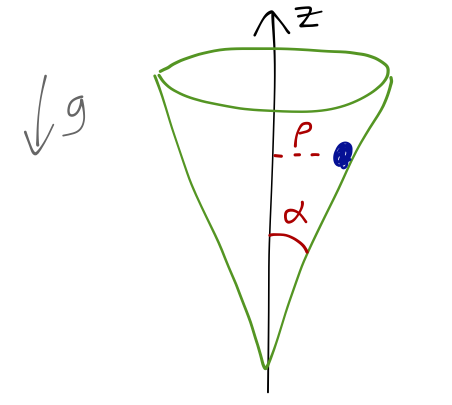
Let's start by finding the Lagrangian. Clearly, cylindrical coordinates are the way to go here; the Lagrangian is then
\[ \begin{aligned} \mathcal{L} = \frac{1}{2} m (\dot{\rho}^2 + \dot{z}^2 + \rho^2 \dot{\theta}^2) - mgz. \end{aligned} \]
Since our particle is stuck to the surface of the cone, we have a constraint between \( z \) and \( \rho \),
\[ \begin{aligned} \rho = z \tan \alpha. \end{aligned} \]
Plugging back in to eliminate \( z \), we have (since \( \dot{z} = \dot{\rho} \cot \alpha \))
\[ \begin{aligned} \mathcal{L} = \frac{1}{2} m (\dot{\rho}^2 (1 + \cot^2 \alpha) + \rho^2 \dot{\theta}^2) - mg \rho \cot \alpha. \end{aligned} \]
Now, we take derivatives to find the two generalized momenta:
\[ \begin{aligned} p_\theta = \frac{\partial \mathcal{L}}{\partial \dot{\theta}} = m\rho^2 \dot{\theta} \\ p_\rho = \frac{\partial \mathcal{L}}{\partial \dot{\rho}} = m \dot{\rho} (1 + \cot^2 \alpha). \end{aligned} \]
These are nice and easy to solve for \( \dot{\rho} \) and \( \dot{\theta} \); we just divide through by the constant stuff. Moreover, our generalized coordinates are independent of time, so we know we can write \( \mathcal{H} = T + U \). So, taking these and plugging back in to the kinetic energy \( T \), we have
$$ \begin{aligned} \mathcal{H} = \frac{1}{2} m \left(\frac{p_\rho}{m (1+\cot2\alpha)}\right)2 (1 + \cot^2 \alpha) \
- \frac{1}{2} m \rho^2 \left(\frac{p_\theta2}{m\rho2}\right)^2 + mg \rho \cot \alpha
= \frac{p_\rho^2}{2m (1 + \cot^2 \alpha)} + \frac{p_\theta2}{2m\rho2} + mg \rho \cot \alpha. \end{aligned} $$
Hamilton's equations for \( \theta \) are pretty simple:
\[ \begin{aligned} \dot{p}_\theta = -\frac{\partial \mathcal{H}}{\partial \theta} = 0 \\ \dot{\theta} = \frac{\partial \mathcal{H}}{\partial p_\theta} = \frac{p_\theta}{m\rho^2}. \end{aligned} \]
So the second equation gave us back the definition of \( p_\theta \), and the first told us that \( p_\theta \) is constant. Because \( \dot{p}_{\theta} = 0 \), we say that \( \theta \) is an ignorable coordinate. Note that this does not mean that \( \theta \) is a constant, too; in fact, we can see that \( \dot{\theta} \) is generally non-zero and can even change, as long as \( \rho \) evolves in time.
Given these complications, what does "ignorable" even mean? We know two things about \( \theta \): that \( \partial \mathcal{H} / \partial \theta = 0 \), and that \( p_\theta \) is a constant. But this means that the Hamiltonian itself can be written as
\[ \begin{aligned} \mathcal{H} = \mathcal{H}(\rho, p_\rho, p_\theta) \end{aligned} \]
and \( p_\theta \) is a constant; in other words, the Hamiltonian is now a function only of two variables, not four! Explicitly, if we write out the other two equations for \( \rho \), we find
\[ \begin{aligned} \dot{p}_\rho = -\frac{\partial \mathcal{H}}{\partial \rho} = \frac{p_\theta^2}{m\rho^3} - mg \cot \alpha \\ \dot{\rho} = \frac{\partial \mathcal{H}}{\partial p_\rho} = \frac{p_\rho}{m (1 + \cot^2 \alpha)}. \end{aligned} \]
This describes an equivalent one-dimensional problem, because the only variables in these equations that are time-dependent are \( \rho \) and \( p_\rho \); we could combine them into a single second-order differential equation for \( \rho \). Taking the derivative of the second equation,
\[ \begin{aligned} \ddot{\rho} = \frac{1}{m(1+\cot^2 \alpha)} \dot{p}_\rho = \frac{1}{m(1+\cot^2 \alpha)} \left( \frac{p_\theta^2}{m\rho^3} - mg \cot \alpha \right). \end{aligned} \]
This is a hard equation to solve directly. But there's another trick up our sleeve; we can notice that the Hamiltonian can be rewritten in the form
\[ \begin{aligned} \mathcal{H}_{1d} = \frac{p_\rho^2}{2\mu} + U_{\textrm{eff}}(\rho) \end{aligned} \]
where
\[ \begin{aligned} \mu = m (1 + \cot^2 \alpha) = m/\sin^2 \alpha \\ U_{\textrm{eff}} = \frac{p_\theta^2}{2m\rho^2} + mg\rho \cot \alpha. \end{aligned} \]
We have done this trick before, of course, when we first solved the central-force motion problem. But notice that it is much easier in the Hamiltonian approach. All we have to do is look at \( \mathcal{H} \), notice that \( p_\theta \) is conserved since there's no \( \theta \) dependence, and just read off the equivalent one-dimensional problem for \( \rho \). If instead we tried to use the Lagrangian, we would have to be careful when taking the equations of motion and trying to plug back in to find the equivalent problem, because there are crucial minus signs lurking!
The Hamiltonian approach also easily generalizes to many ignorable coordinates: we just identify them (by noticing that \( \partial \mathcal{H} / \partial q_i = 0 \)), and then immediately focus on solving for the remaining non-ignorable coordinates.
(This arises from the fact that our assumption in deriving the Lagrangian equations of motion was that \( \dot{\theta} \) was held fixed at the endpoints of the path; but as we've seen, this isn't the same as \( p_\theta \) staying fixed. The Hamiltonian approach, on the other hand, treats momentum and coordinate as separate variables, so we don't have to worry about this subtlety.)
To finish our solution, notice that we can draw the effective potential for \( \alpha > 0 \) and \( p_\theta > 0 \), and it looks like this:
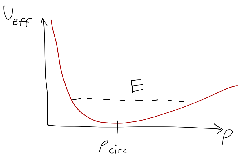
Clearly, any orbit within the cone is bound; at the minimum of the potential, we find the usual circular orbit:
\[ \begin{aligned} \frac{dU_{\textrm{eff}}}{d\rho} = -\frac{p_\theta^2}{m\rho^3} + mg \cot \alpha = 0 \\ \Rightarrow \rho_{\textrm{circ}} = \left( \frac{p_\theta^2 \tan \alpha}{m^2 g} \right)^{1/3}. \end{aligned} \]
We could also try to make a phase-space plot of \( \rho \) and \( p_\rho \), but we already know from the effective potential analysis that it won't be very interesting; for any initial point \( (\rho, p_\rho) \) we'll just find periodic motion between the minimum and maximum \( \rho \) values given by setting \( E = U_{\textrm{eff}}(\rho) \).
Example: A springy Atwood's machine
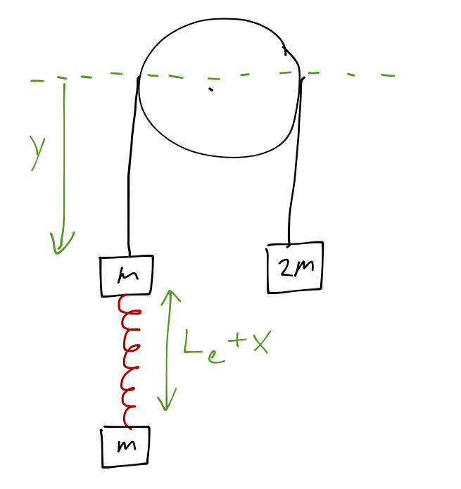
The setup is as drawn in the sketch. The gravitational potential isn't too hard to write down:
\[ \begin{aligned} U_g = (2m)gy - mgy - mg(x+y) = -mgx. \end{aligned} \]
We're given the equilibrium length \( L_e \) of the spring to work with; at equilibrium the spring and gravitational forces balance, i.e.
\[ \begin{aligned} k(L_e - L_0) = mg \end{aligned} \]
where \( L_0 \) is the unstretched length of the spring. The extension of the spring in total is thus
\[ \begin{aligned} (x + L_e) - L_0 = x + \frac{mg}{k}. \end{aligned} \]
We can plug back in to find the spring potential,
\[ \begin{aligned} U_k = \frac{1}{2} k \left(x + \frac{mg}{k}\right)^2 \\ = \frac{1}{2} kx^2 + mgx + (\textrm{const}). \end{aligned} \]
Despite the rather complicated setup, our total potential energy is extremely simple, and doesn't even depend on gravity: the \( mgx \) terms cancel, and we simply find
\[ \begin{aligned} U = \frac{1}{2} kx^2. \end{aligned} \]
For the kinetic energy, we have
\[ \begin{aligned} T = \frac{1}{2} (2m) \dot{y}^2 + \frac{1}{2} m \dot{y}^2 + \frac{1}{2} m (\dot{x} + \dot{y})^2 = \frac{1}{2} m \left[ 3\dot{y}^2 + (\dot{x} + \dot{y})^2\right]. \end{aligned} \]
Clearly in this case, the coordinates don't depend explicitly on time. (The vertical position of the lowest block depends on both \( x \) and \( y \), but that's perfectly fine!) So we can definitely write the Hamiltonian using the shortcut form \( \mathcal{H} = T + U \). The momenta are defined by
\[ \begin{aligned} p_x = \frac{\partial \mathcal{L}}{\partial \dot{x}} = m (\dot{x} + \dot{y}) \\ p_y = \frac{\partial \mathcal{L}}{\partial \dot{y}} = m (4\dot{y} + \dot{x}) \end{aligned} \]
which we can invert to get
\[ \begin{aligned} \dot{x} + \dot{y} = \frac{p_x}{m} \\ \dot{y} = \frac{1}{3m} (p_y - p_x). \end{aligned} \]
Thus the Hamiltonian turns out to be
\[ \begin{aligned} \mathcal{H} = \frac{1}{2m} \left[ \frac{(p_x - p_y)^2}{3} + p_x^2 \right] + \frac{1}{2}kx^2. \end{aligned} \]
Since \( \partial \mathcal{H} / \partial y = 0 \), we see that \( y \) is ignorable, and thus \( p_y \) is a constant. The good news is that this reduces our problem to an equivalent one-dimensional one. The bad news is that we can't rewrite it using an effective potential, because for \( p_y \neq 0 \) there is a term linear in \( p_x \). But as a special case, if we start the apparatus from rest (\( \dot{x}(0) = \dot{y}(0) = 0 \)), then \( p_y = 0 \) and I simply have
\[ \begin{aligned} \mathcal{H} = \frac{2p_x^2}{3m} + \frac{1}{2} kx^2 \end{aligned} \]
This is an effective one-dimensional problem for a simple harmonic oscillator, with mass \( \mu = 3m/4 \). So we can immediately see that when the system starts from rest, it will undergo simple harmonic motion in \( x \) at a frequency \( \omega^2 = k/\mu = 4k/3m \):
\[ \begin{aligned} x(t) = x_0 \cos (\sqrt{4k/3m}t) \end{aligned} \]
Once again, don't forget that \( y \) does change even though \( p_y \) is zero for all time! I can see this from the fact that \( \dot{y} \) depends on both \( p_y \) and \( p_x \). If we go back and plug in to Hamilton's equations we will find that \( y \) also oscillates at the same frequency.
What if we actually wanted to solve for \( x \)? We haven't written Hamilton's equations yet: for \( p_x \), we have
\[ \begin{aligned} \dot{p}_x = -\frac{\partial \mathcal{H}}{\partial x} = -kx \\ \dot{x} = \frac{\partial \mathcal{H}}{\partial p_x} = \frac{4p_x - p_y}{3m} \end{aligned} \]
or taking the derivative of the second equation,
\[ \begin{aligned} \ddot{x} = \frac{4\dot{p}_x}{3m} = -\frac{4k}{3m} x. \end{aligned} \]
So the result is actually quite simple: even if \( p_y \neq 0 \), \( x \) still undergoes simple harmonic motion at the same frequency.