Concept: Angular momentum of rigid objects
We now have all of the pieces to look at the details of how rotational motion of a rigid object gives rise to (internal) kinetic energy and angular momentum. Let's start simple, with rotation about a fixed axis: imagine a steel rod as a physical axis, onto which we thread some arbitrary solid object.
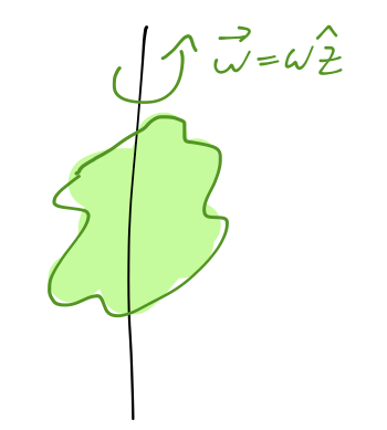
The rotation axis is set to be \( \vec{\omega} = \omega \hat{z} \). For any point within the object, we write its position as \( \vec{r}_\alpha \), with origin at the CM. Since the object is rigid, in a frame rotating with the object every point is at rest: the velocity of a point due to the rotation is thus
\[ \begin{aligned} \dot{\vec{r}}_\alpha = \vec{\omega} \times \vec{r}_\alpha \\ = -\omega y_\alpha \hat{x} + \omega x_\alpha \hat{y}. \end{aligned} \]
The angular momentum is then
\[ \begin{aligned} \vec{L}_\alpha = m_\alpha \vec{r}_\alpha \times \dot{\vec{r}}_\alpha \\ = m_\alpha \left| \begin{array}{ccc} \hat{x}&\hat{y}&\hat{z} \\ x_\alpha & y_\alpha & z_\alpha \\ -\omega y_\alpha & \omega x_\alpha & 0 \end{array} \right| \\ = m_\alpha \omega \left( -z_\alpha x_\alpha \hat{x} - z_\alpha y_\alpha \hat{y} + (x_\alpha^2 + y_\alpha^2) \hat{z} \right). \end{aligned} \]
To calculate the total angular momentum of the object, we sum over all of the component angular momenta. Let's do the \( z \) component first:
\[ \begin{aligned} L_z = \sum_\alpha (L_{\alpha,z}) = \sum_\alpha m_\alpha \omega (x_\alpha^2 + y_\alpha^2) \\ = \left(\sum_\alpha m_\alpha r_\alpha^2\right) \omega \\ = I_z \omega \end{aligned} \]
In other words, the angular momentum about the axis of rotation is proportional to \( \omega \), and the proportionality is given by the sum over (mass) x (distance from axis)\( ^2 \). This is exactly the moment of inertia about the \( z \)-axis, as you learned it in freshman physics!
Moreover, notice that the kinetic energy of the rotating object is equal to
\[ \begin{aligned} T = \frac{1}{2} \sum_\alpha m_\alpha \dot{\vec{r}}_\alpha^2 \\ = \frac{1}{2} \sum_\alpha m_\alpha (\omega^2 y_\alpha^2 + \omega^2 x_\alpha^2) \\ = \frac{1}{2} \sum_\alpha m_\alpha r_\alpha^2 \omega^2 = \frac{1}{2} I_z \omega^2. \end{aligned} \]
This is another formula you've seen before (and we've used in Lagrangian mechanics.) Here's the part that you haven't seen before: what about the \( x \) and \( y \) components of \( \vec{L} \)? We can calculate those too:
\[ \begin{aligned} L_x = \sum_\alpha m_\alpha (-z_\alpha x_\alpha \omega) = I_x \omega \\ L_y = \sum_\alpha m_\alpha (-z_\alpha y_\alpha \omega) = I_y \omega. \end{aligned} \]
For something simple like a uniform cylinder rotating around its symmetry axis, these components vanish identically: at any \( z \), for every \( x_\alpha \) there is an equal mass at \( -x_\alpha \) to cancel it in the sum. But for an arbitrary object, these moments don't have to be zero!
This brings us to a very, very important point: \( \vec{L} \) and \( \vec{\omega} \) do not necessarily point in the same direction. The equation \( \vec{L} = I \vec{\omega} \) (where \( I \) is a numerical constant), as you learned it in freshman physics, is obviously not true in all scenarios; in general, \( I \) must be a matrix, an operator which can transform one vector into another.
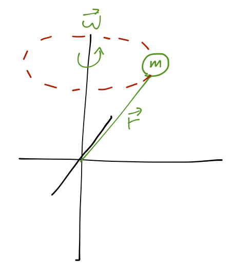
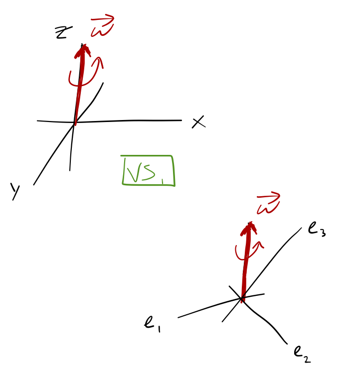
Let's drive this home with an example. Consider a single mass attached to a massless, pivoting rod, at a fixed angle to the \( z \)-axis. The mass and rod pivot about the \( z \)-axis with constant angular speed \( \vec{\omega} \).
Clicker Question
What is the direction of \( \vec{L} \) at this moment?
A. Up
B. Into the page
C. Left
D. Up and left
E. Down and right
Answer: D
Use the right-hand rule: \( \vec{L} = m \vec{r} \times \vec{v} \), and \( \vec{r} \) and \( \vec{v} \) are perpendicular (\( \vec{v} \) points into the page.) So \( \vec{L} \) points up and to the left.
Clicker Question
What happens to \( \vec{L} \) and \( \mathbf{I} \) in these coordinates as the mass spins around?
A. \( \vec{L} \) is constant, but \( \mathbf{I} \) changes; no net torque.
B. \( \vec{L} \) and \( \mathbf{I} \) are both constant; no net torque.
C. \( \vec{L} \) changes, because \( \mathbf{I} \) changes; no net torque.
D. \( \vec{L} \) and \( \mathbf{I} \) both change; there is a net torque.
E. \( \vec{L} \) changes, but \( \mathbf{I} \) is constant; there is a net torque.
Answer: D
Let's start by answering the basic question: does \( \vec{L} \) change? If the system rotates around 180 degrees, we can see that now (with \( \vec{v} \) pointing out of the page) \( \vec{L} \) points up and to the right, instead. So \( \vec{L} \) is changing with the motion!
Although we're used to thinking of moments of inertia as a static property of an object, it should be easy for you to see that \( \mathbf{I} \) is changing with time, too! Since we just have a single point mass, our sums for \( \mathbf{I} \) above collapse to a single term. In particular, we see that at the starting point drawn, \( I_x = mxz \neq 0 \), while \( I_y = myz = 0 \). On the other hand, if we now look after a 90-degree rotation, we will find \( I_x = 0 \) and \( I_y \neq 0 \). In fact, if \( \vec{L} \) is changing and \( \vec{\omega} \) is constant, the relationship \( \vec{L} = \mathbf{I} \vec{\omega} \) tells us that \( \mathbf{I} \) has to be changing with time.
This narrows our options down to C and D; the answer is D because there is, in fact, a net torque. If we recall that \( \vec{\Gamma} = \dot{\vec{L}} \), we know that as long as \( \vec{L} \) is changing, there must be a net torque. Where does it come from? There is one force in this system, provided by the rod connecting our mass to the origin; the rod is providing the centripetal force to keep the mass moving in a circular path. This force points directly towards the rotational axis, and not along \( \vec{r} \), so the torque \( \vec{r} \times \vec{F} \) is indeed non-zero.
Notice, by the way, that angular momentum and torque depend on our coordinate choice! If we took the origin of our coordinate system to be at the center of the circle around which our mass is moving, instead of where the rod is attached, then we would find zero torque and constant \( \vec{L} \) in the \( z \)-direction. Both of these statements are perfectly consistent with the motion we see, in their respective coordinate systems. Remember that as we go through this subject!
What we've seen is that even in a simple case like this, it's often true that \( \vec{L} \) and \( \vec{\omega} \) are not aligned. In general, this doesn't require the presence of torque, nor does it require that \( \vec{\omega} \) remain fixed. In fact, this scenario is somewhat unrealistic; it's much more common for us to encounter motion with no torques in which \( \vec{L} \) is fixed, but \( \vec{\omega} \) can still change. If you throw your copy of Taylor into the air (note: do this at your own risk!) you will see it tumbling around in the absence of any forces, which is exactly this sort of motion.
Of course, books are expensive and don't stay in the air very long, so how about we watch a video from an astronaut on the International Space Station instead?
Video: Spinning a deck of cards in space!
Formula: The inertia tensor
Last time, we started looking at the motion of collections of particles, and found that for a number of very interesting quantities, there is a clean division between the motion of the center of mass (CM), and the motion relative to the CM. In particular, we saw that
\[ \begin{aligned} T = T_{CM} + T_{\rm rel} \\ U = U_{CM} + U_{\rm rel} \\ \vec{L} = \vec{L}_{CM} + \vec{L}_{\rm rel}. \end{aligned} \]
We specialized further to rigid bodies, which are collections in which none of the particles move relative to each other; this allows us to treat \( U_{\rm rel} \) as an ignorable constant, and leaves rotation as the only possible relative motion contributing to \( T \) and \( \vec{L} \).
After that, we studied motion about a fixed axis, say \( \vec{\omega} = \omega \hat{z} \), and derived the familiar formulas
\[ \begin{aligned} L_z = I_z \omega \\ T_{\textrm{rot}} = \frac{1}{2} I_z \omega^2. \end{aligned} \]
Here \( I_z \) is the familiar moment of inertia for rotation about this axis. The moment of inertia tells us how resistant the object is to changes in rotational velocity; the larger \( I_z \), the more energy we need to put in to increase \( \omega \) and \( L_z \). (The moment of inertia plays the same role in rotation that the ordinary mass \( m \) does in linear motion.)
But we found that in general, these are simplified relations that only hold for highly symmetric objects! As we saw, it's often the case that \( \vec{L} \) and \( \vec{\omega} \) don't even point in the same direction. This means that the moment of inertia must in fact be an operator which can rotate one vector (\( \vec{\omega} \)) into another (\( \vec{L} \)); in other words, it's a matrix, \( \mathbf{I} \).
Rotation about any axis
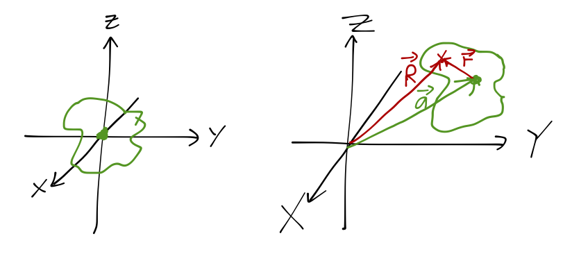
Now let's move on to rotation about an arbitrary axis, and see the general form of this inertia matrix. Take a general rotation vector \( \vec{\omega} = (\omega_x, \omega_y, \omega_z) \); the rotation is taken with respect to the center of mass and the body is otherwise stationary, so the speed of each particle is
\[ \begin{aligned} \dot{\vec{r}}_\alpha = \vec{\omega} \times \vec{r}_\alpha. \end{aligned} \]
Thus, the angular momentum carried by each particle is
\[ \begin{aligned} \vec{L}_\alpha = m_\alpha \vec{r}_\alpha \times (\vec{\omega} \times \vec{r}_\alpha). \end{aligned} \]
Expanding out both cross products in turn is tedious, so I'll just skip to the result, which can be written in matrix form:
\[ \begin{aligned} \vec{L}_\alpha = m_\alpha \left( \begin{array}{ccc} y_\alpha^2 + z_\alpha^2 & -x_\alpha y_\alpha & -x_\alpha z_\alpha \\ -x_\alpha y_\alpha & x_\alpha^2 + z_\alpha^2 & -y_\alpha z_\alpha \\ -x_\alpha z_\alpha & -y_\alpha z_\alpha & x_\alpha^2 + y_\alpha^2 \end{array} \right) \left( \begin{array}{c} \omega_x \\ \omega_y \\ \omega_z \end{array} \right). \end{aligned} \]
This is a compact way of writing three equations, one for each component of \( \vec{L}_\alpha \). Notice that setting \( \vec{\omega} = \omega \hat{z} \) gives us the fixed-axis result we found last time. Once again, to get the total angular momentum, we sum over the individual particles \( \alpha \), and we can pull \( \vec{\omega} \) out of the sum, so finally we have:
\[ \begin{aligned} \vec{L} = \mathbf{I} \vec{\omega} \end{aligned} \]
which defines the inertia matrix or inertia tensor,
Definition: the inertia tensor
\[ \begin{aligned} \mathbf{I} = \sum_\alpha m_\alpha \left( \begin{array}{ccc} y_\alpha^2 + z_\alpha^2 & -x_\alpha y_\alpha & -x_\alpha z_\alpha \\ -x_\alpha y_\alpha & x_\alpha^2 + z_\alpha^2 & -y_\alpha z_\alpha \\ -x_\alpha z_\alpha & -y_\alpha z_\alpha & x_\alpha^2 + y_\alpha^2 \end{array} \right) \\ {\rm or:}\\ \mathbf{I} = \int dV\ \rho(x,y,z) \left( \begin{array}{ccc} y^2 + z^2 & -x y & -x z \\ -x y & x^2 + z^2 & -y z \\ -x z & -y z & x^2 + y^2 \end{array} \right). \end{aligned} \]
The second version of this just replaces the sum with an integral, for an object described by some continuous density function \( \rho(x,y,z) \). Don't be confused by the "integral of a matrix"; the components of the matrix are all separate, so you can think of writing nine separate integrals inside the matrix, I just wrote it like this to save space.
Notice that this is a symmetric matrix; that has some important implications, but one thing we can see immediately is that although it's a 3x3 matrix, there are only six independent entries we have to find.
It's very important to remember that this formula defines the moments of inertia only for rotational axes which pass through the origin of the coordinate system, \( x=y=z=0 \). This special point through which all rotational axes pass is called the pivot point. If we want to calculate rotation around an axis which doesn't pass through the origin, we have to shift our coordinates to use the formula above. Remember, angular momentum is sensitive to where we put our coordinates! (The actual motion of the system that we find in the end will, of course, be independent of coordinate choices, but as we saw last time, statements like "\( \vec{L} \) is constant" do depend on coordinates.)
By the way, it shouldn't surprise you that the equation for kinetic energy is modified too! The derivation is a bit of a pain, so I'll just tell you that the general formula is
\[ \begin{aligned} T = \frac{1}{2} \vec{\omega} \cdot \vec{L} = \frac{1}{2} \vec{\omega}^T \mathbf{I} \vec{\omega}. \end{aligned} \]
You can see that this reproduces the simplified formula \( T = \frac{1}{2} I \omega^2 \), which is valid only for rotation that keeps \( \vec{\omega} \) and \( \vec{L} \) parallel.
Tensors and index notation
It's worth making a brief detour here into index notation, which will give us a much nicer-looking formula for the inertia tensor. We know that we can break any vector down into its components:
\[ \begin{aligned} \vec{a} = a_x \hat{x} + a_y \hat{y} + a_z \hat{z}. \end{aligned} \]
Here we've written the components as \( a_i \), where \( i \) is a placeholder for any of \( x,y,z \). (By convention, latin indices \( i,j,k... \) are used for spatial coordinates.) Index notation gives us a compact way of rewriting certain formulas in terms of components. For example, the dot product:
\[ \begin{aligned} \vec{a} \cdot \vec{b} = a_x b_x + a_y b_y + a_z b_z \\ = \sum_i a_i b_i. \end{aligned} \]
This notation is easily extended to larger objects. The inertia tensor itself is a matrix, so we need two indices \( ij \) to write out its 9 components. Which entry is which, in this notation? Well, we can write out matrix-vector products as sums over indices. These two equations have the same meaning:
\[ \begin{aligned} \vec{L} = \mathbf{I} \vec{\omega} \\ L_i = \sum_j I_{ij} \omega_j. \end{aligned} \]
So, for example, the \( x \)-component of \( \vec{L} \) is given by
\[ \begin{aligned} L_x = I_{xx} \omega_x + I_{xy} \omega_y + I_{xz} \omega_z \\ \left( \begin{array}{c} L_x \\ ... \\ ... \end{array} \right) = \left( \begin{array}{ccc} I_{xx} & I_{xy} & I_{xz} \\ &...& \\ &...& \end{array}\right) \left( \begin{array}{c} \omega_x \\ \omega_y \\ \omega_z \end{array} \right) \end{aligned} \]
This is the dot product of the column vector \( \vec{\omega} \) with the first row of \( \mathbf{I} \), so we see that the first index labels the row, and the second index is the column.
With this notation set up, we can write a much more compact formula for the inertia tensor:
Inertia tensor (compact form)
\[ \begin{aligned} I_{ij} = \int\ dV\ \rho(x,y,z) (r^2 \delta_{ij} - r_i r_j) \end{aligned} \]
where \( r_i = (r_x, r_y, r_z) = (x, y, z) \), and \( r^2 = x^2 + y^2 + z^2 \) (this is all still in rectangular coordinates!) I have introduced a special symbol here known as the Kronecker delta symbol, which is equal to \( 1 \) if the two indices are equal and \( 0 \) otherwise:
\[ \begin{aligned} \delta_{ij} = \begin{cases} 1, & i = j;\\ 0, & i \neq j. \end{cases} \end{aligned} \]
In matrix form, the Kronecker delta is just the identity matrix. We could go much further with index notation; for example, I could define the cross product using a different special tensor. But for now, we only really wanted the compact version of \( \mathbf{I} \), so let's move on.
By the way, I haven't really defined the term tensor. A tensor is a mathematical object that is sensitive to coordinate changes in a certain way. Consider the simple change of coordinates from rectangular to cylindrical:
\[ \begin{aligned} x = r \cos \theta \\ y = r \sin \theta \\ z = z \end{aligned} \]
If we're just interested in a quantity like the kinetic energy, then we just substitute in one coordinate for another using these equations: \( \dot{x}^2 + \dot{y}^2 \) becomes \( \dot{r}^2 + r^2 \dot{\theta}^2 \), for example. But if we have a vector and we want to change coordinates; we have to go further, and account for the change of basis vectors from \( \hat{x}, \hat{y} \) to \( \hat{r}, \hat{\theta} \).
A vector is an example of a tensor, because of this extra sensitivity to the unit vectors in our coordinate change. The "inertia tensor" will also depend on the unit vectors, but in a more complicated way: to fully change coordinates here, we have to identify what \( I_{rr} \) is in terms of the original \( x \) and \( y \) components, and so on. We're not going to deal with coordinate changes of tensors in full generality here; just keep in mind that the inertia matrix isn't just a fixed set of numbers, but that it depends intricately on the definition of our coordinates. I'll continue to say "inertia tensor" since that's standard jargon, but you can just think "inertia matrix".
Formula: The parallel axis theorem
Let's consider two coordinate systems: the first \( \vec{r} = (x,y,z) \) with origin at the center of mass of an arbitrary extended object, and the second \( \vec{R} = (X,Y,Z) \) offset by some distance. As described in \( \vec{R} \), the object is displaced from the origin (but not rotated!) by some constant vector \( \vec{a} \).
As the name implies, the axes of the two coordinate systems are parallel - \( \hat{x} \) and \( \hat{X} \) point in the same direction, and the same for \( y \) and \( z \). We're just displacing the origin. In vector form, the coordinates are related as
\[ \begin{aligned} \vec{R} = \vec{a} + \vec{r}. \end{aligned} \]
Note that \( \vec{a} \) points towards the center of mass - the direction is important! It's a straightforward exercise in algebra to write down the inertia tensor in one coordinate system and translate it to the other coordinates: just write \(R_i = r_i + a_i\) and recognize that anything which looks like \(\sum_{\alpha} m_\alpha \vec{r}_\alpha\) is zero, since it's the position of the CM in the CM coordinates.
I'll skip the algebra here, and just give you the answer. If \( I_{ij} \) is the inertia tensor calculated in CM coordinates, and \( J_{ij} \) is the tensor in the displaced coordinates, then:
\[ \begin{aligned} J_{ij} = I_{ij} + M(a^2 \delta_{ij} - a_i a_j). \end{aligned} \]
Let's try on the cube! Recall that the CM inertia tensor was
\[ \begin{aligned} \mathbf{I} = Mb^2 \left( \begin{array}{ccc} 1/6 & 0 & 0 \\ 0 & 1/6 & 0 \\ 0 & 0 & 1/6 \end{array} \right) \end{aligned} \]
If instead we want the tensor about one corner of the cube, the displacement vector is \( \vec{a} = (b/2, b/2, b/2) \), so \( a^2 = (3/4) b^2 \). We can construct the difference as a matrix: the on-diagonal components are
\[ \begin{aligned} M \left[\frac{3}{4} B^2 - \left(\frac{1}{2} b\right)\left(\frac{1}{2} b\right) \right] = \frac{1}{2} M b^2 \end{aligned} \]
and off-diagonal,
\[ \begin{aligned} M \left[-\left(\frac{1}{2} b\right)\left(\frac{1}{2} b\right) \right] = -\frac{1}{4} M b^2 \end{aligned} \]
so the shifted inertia tensor is
\[ \begin{aligned} \mathbf{J} = Mb^2 \left( \begin{array}{ccc} 1/6 & 0 & 0 \\ 0 & 1/6 & 0 \\ 0 & 0 & 1/6 \end{array} \right) + Mb^2 \left( \begin{array}{ccc} 1/2 & -1/4 & -1/4 \\ -1/4 & 1/2 & -1/4 \\ -1/4 & -1/4 & 1/2 \end{array} \right) \\ = Mb^2 \left( \begin{array}{ccc} 2/3 & -1/4 & -1/4 \\ -1/4 & 2/3 & -1/4 \\ -1/4 & -1/4 & 2/3 \end{array} \right) \end{aligned} \]
exactly matching the result from calculating it the direct way (we'll do this as an example.)
Concept: Rotational motion and principal axes
Back to motion of a rotating object:
\[ \begin{aligned} \vec{\Gamma} = \dot{\vec{L}}. \end{aligned} \]
where I'll remind you that \( \vec{\Gamma} = \vec{r} \times \vec{F} \). As we saw, in a fixed set of coordinates, in general the right-hand side of this equation splits into two components:
\[ \begin{aligned} \dot{\vec{L}} = \dot{\mathbf{I}} \vec{\omega} + \mathbf{I} \dot{\vec{\omega}}. \end{aligned} \]
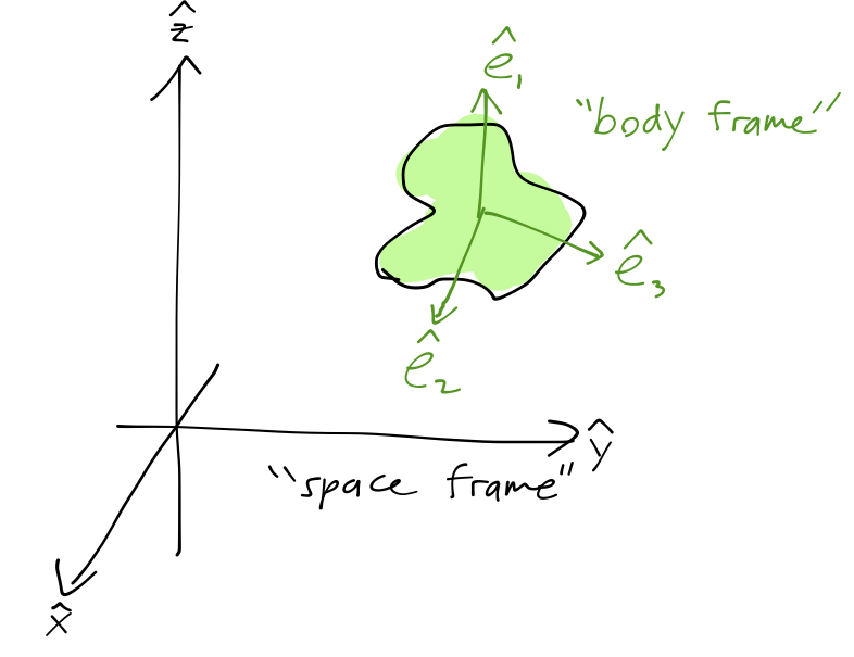
In principle, we can describe the motion by calculating \( \mathbf{I}(t) \). Of course, computing the inertia tensor once for a static object is already a pain, and we really don't want to evaluate those integrals for a completely arbitrary orientation of the object. A better alternative is to work in a body coordinate system, one which rotates along with the object itself. This forces the inertia tensor to remain fixed.
The body frame is, of course, non-inertial, so we still find that \( \vec{\omega} \) can change even with no external torques, because within the rotating frame \( \vec{L} \) does change with time (there are fictitious torques, if you like.) As always, these pictures in different frames of reference are identical in terms of the actual motion.
Recall that when changing from a fixed frame (here usually called the space frame) to a rotating frame (the body frame), the time derivative of a vector changes. So for angular momentum,
\[ \begin{aligned} \vec{\Gamma} = \left( \frac{d\vec{L}}{dt} \right)_{\textrm{space}} \end{aligned} \]
becomes
\[ \begin{aligned} \vec{\Gamma} = \left( \frac{d\vec{L}}{dt} \right)_{\textrm{body}} + \vec{\omega} \times \vec{L}, \end{aligned} \]
or since we've specifically chosen the body frame so that \( \mathbf{I} \) is constant,
\[ \begin{aligned} \vec{\Gamma} = \mathbf{I} \dot{\vec{\omega}} + \vec{\omega} \times \vec{L}. \end{aligned} \]
Warning: it may be confusing to think about expanding the angular velocity vector \( \vec{\omega} \) in the body frame. After all, the body frame is co-rotating with the object, so there is no rotating left in the body frame, right?
We have to update our thinking about rotating frames, in which we've always set up our coordinates to orient the rotation vector \( \vec{\omega} \) with one of the axes. But as we'll see shortly, the best choice of coordinate axes to use for the body frame is not always aligned with the rotation vector - it will be dictated by the geometry of our object.
There's nothing wrong with defining a rotating coordinate system that isn't aligned with \( \vec{\omega} \), but if we set up our coordinates like this, then the components of \( \vec{\omega} \) will generally change as the coordinate system spins around. This is clear if \( \vec{\omega} \) is fixed in the space frame; it's a little less clear how to understand what's happening if \( \vec{\omega} \) changes there too, but we'll see some examples soon.
Principal axes
In general, this equation is very complicated; in fact it's a set of three equations, and since \( \vec{L} = \mathbf{I} \vec{\omega} \) in general has nine non-zero entries, every equation depends on all three components of \( \vec{\omega} \). However, in the special case that \( \mathbf{I} \) is diagonal, the equations are much more simple. But diagonal inertia tensors have only arisen from special objects with a high degree of symmetry so far. Is the motion of a less symmetric object hopelessly complicated? The answer is no!
Although in general the inertia matrix \( \mathbf{I} \) can give \( \vec{L} \) oriented in a different direction from \( \vec{\omega} \), in some cases we have seen that the two vectors do point in the same direction. If we can identify that
\[ \begin{aligned} \vec{L} = \lambda \vec{\omega}, \end{aligned} \]
for some constant \( \lambda \) and some choice of \( \vec{\omega} \), then we say that \( \vec{\omega} \) points along a principal axis of the corresponding rigid body, and the factor \( \lambda \) is said to be the corresponding principal moment.
Clicker Question
_Suppose we calculate a diagonal inertia matrix for an object in some coordinate system, with \( \lambda_1 > \lambda_2 > \lambda3 \). What are the principal axes?
A. Any group of three orthogonal axes
B. (1,0,0), (0,1,0), and (0,0,1)
C. \( (\lambda_1, \lambda_2, \lambda_3) \) and two perpendicular vectors
D. Impossible to tell without more info
Answer: B
If the inertia matrix is diagonal, then if \( \vec{\omega} \) points along any of the coordinate axes, then \( \mathbf{I} \vec{\omega} \) points in the same direction. So the principal axes are the coordinate axes, if \( \mathbf{I} \) is diagonal.
Clicker Question
Now we calculate the inertia matrix of a second object, and it is not diagonal. What are the principal axes?
A. Any group of three orthogonal axes
B. (1,0,0), (0,1,0) and (0,0,1)
C. \( (\lambda_1, \lambda_2, \lambda_3) \) is principal, where \( \lambda \) are the eigenvalues of \( \mathbf{I} \)
D. \( \hat{e}_1 \), \( \hat{e}_2 \), and \( \hat{e}_3 \), where \( \hat{e} \) are the eigenvectors of \( \mathbf{I} \)
E. Impossible to tell
Answer: D
The condition for \( \vec{\omega} \) to point along a principal axis can be rewritten as
\[ \begin{aligned} \mathbf{I} \vec{\omega} = \lambda \vec{\omega}. \end{aligned} \]
This is the eigenvalue/eigenvector equation for the inertia matrix. The eigenvalues of the matrix are \( \lambda \), the principal moments; their corresponding eigenvectors give the principal axes.
So the eigenvectors of \( \mathbf{I} \) for any object point in a direction along which \( \vec{L} \) is proportional to \( \vec{\omega} \). In coordinates described by the eigenvectors, then, the inertia matrix is diagonal!
Because the inertia tensor is a real, symmetric matrix, there will always be three perpendicular principal axes that we can find. This is worth stating clearly: for any rigid body and any point \( O \), there are three mutually perpendicular prinicpal axes passing through \( O \), such that the inertia tensor of the body along these axes is diagonal.
The principal axes automatically give us a "clever" choice of coordinates for the body frame: when we use the principal axes as our coordinate directions, we always have a diagonal inertia tensor, and the equation of motion can be written in a simplified form.
Formula: Euler's equations
Now that we know we can always find a set of principal axes and diagonalize \( \mathbf{I} \), let's see exactly how the equation of motion
\[ \begin{aligned} \vec{\Gamma} = \mathbf{I} \dot{\vec{\omega}} + \vec{\omega} \times \vec{L} \end{aligned} \]
simplifies in this case. The cross product on the right becomes
\[ \begin{aligned} \vec{\omega} \times \vec{L} = \vec{\omega} \times \left( \begin{array}{ccc} \lambda_1 & 0 & 0 \\ 0 & \lambda_2 & 0 \\ 0 & 0 & \lambda_3 \end{array} \right) \left( \begin{array}{c} \omega_1 \\ \omega_2 \\ \omega_3 \end{array} \right) = \left| \begin{array}{ccc} \hat{e_1} & \hat{e_2} & \hat{e_3} \\ \omega_1 & \omega_2 & \omega_3 \\ \lambda_1 \omega_1 & \lambda_2 \omega_2 & \lambda_3 \omega_3 \end{array} \right|. \end{aligned} \]
(where \( \hat{e_i} \) are the unit vectors of my three body-frame coordinate directions \( 1,2,3 \), pointing along the principal axes of the object.)
Thus, we find in the body frame the following three equations:
Euler's equations:
\[ \begin{aligned} \lambda_1 \dot{\omega_1} - (\lambda_2 - \lambda_3) \omega_2 \omega_3 = \Gamma_1 \\ \lambda_2 \dot{\omega_2} - (\lambda_3 - \lambda_1) \omega_3 \omega_1 = \Gamma_2 \\ \lambda_3 \dot{\omega_3} - (\lambda_1 - \lambda_2) \omega_1 \omega_2 = \Gamma_3. \end{aligned} \]
The form of the torque vector \( \vec{\Gamma} \) in body-frame coordinates tends to be messy, although we'll deal with some special cases. First, let's discuss what happens when there are no torques, so \( \vec{\Gamma} = 0 \).
First observation: if \( \vec{\omega} \) is aligned with one of the body-frame axes, then two of its components are zero, and all of the equations of motion reduce to simply
\[ \begin{aligned} \dot{\omega}_i = 0. \end{aligned} \]
So rotation about any axis is stable in the absence of torques, as long as the inertia tensor is diagonal in our coordinates.
Second observation: for a highly symmetric object like the cube about its CM, all of the differences between moments \( \lambda_i \) are zero, and once again we have \( \dot{\omega}_i = 0 \). So a cube or a sphere will rotate stably for any rotation about its center of mass.
Application: Torque-free motion and tumbling
Now we're finally ready to understand the (torque-free) motion of the deck of cards! As you heard in the video, the motion about certain axes is either stable or unstable. Of course, we just noted that if \( \vec{\omega} \) is perfectly aligned with one of the body-frame axes, then the equations reduce to \( \dot{\omega_i} = 0 \) and the rotation is constant. However, in the real world the alignment is never perfect, so the question of stability is related to what happens when \( \vec{\omega} \) is almost aligned with an axis.
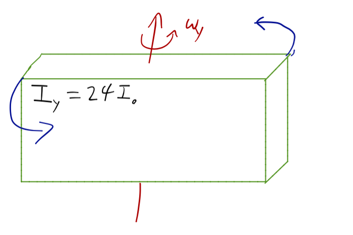
We'll be concrete and use the deck of cards, which is an example of a rectangular prism, a solid with rectangular cross-section in all three directions. The calculation of the moments of inertia for such an object is exactly the same as for the cube about its CM, except that the limits of integration are different for each diagonal component. For example, a standard deck of cards (in the box) has dimensions of about 3.5" x 2.5" x 0.75", or 90 mm x 60 mm x 20 mm.
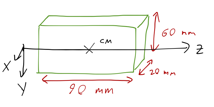
If we let \( \hat{z} \) point in the longest direction and \( \hat{x} \) the shortest, and consider rotation about the CM once again, then the off-diagonal moments are still zero, and the diagonal moments work out to
\[ \begin{aligned} \mathbf{I} \approx M(2\ {\rm cm})^2 \left( \begin{array}{ccc} 33 & 0 & 0 \\ 0 & 24 & 0 \\ 0 & 0 & 11 \end{array} \right). \end{aligned} \]
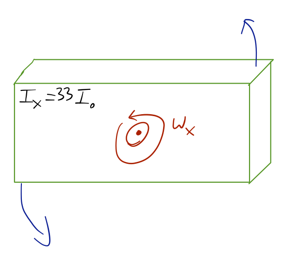
So in our coordinates, the largest moment is for rotation about the \( \hat{x} \) axis, i.e. perpendicular to the broadest face of the deck, like so:
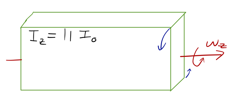
The smallest moment is for rotation about the \( \hat{z} \) axis, perpendicular to the smallest side.
Finally, the intermediate moment corresponds to the in-between side:
We could have predicted this without doing the full calculation; we know that for simple rotation about a chosen axis, where \( \vec{L} \) and \( \vec{\omega} \) are aligned, the moment of inertia is given by integrating over \( \rho r^2 \), with \( r \) the radial distance to that axis. So for an object with constant density, the size of the moment of inertia is given by the size of the cross-sectional area of the object, as viewed from along the rotation axis.
Now, back to Euler's equations. Let's pick an arbitrary axis and call it \( 3 \), without regard to which \( \lambda_i \) is which yet. We suppose that the rotation is nearly in the \( \hat{e}_3 \) direction, so \( \omega_1 \) and \( \omega_2 \) are non-zero but very small. The equation of motion for \( \omega_3 \) (in the absence of torque) is
\[ \begin{aligned} \lambda_3 \dot{\omega_3} = (\lambda_1 - \lambda_2) \omega_1 \omega_2 \approx 0. \end{aligned} \]
since both \( \omega_1 \) and \( \omega_2 \) are small. So \( \omega_3 \) is approximately constant for this motion. The other two equations are
\[ \begin{aligned} \lambda_1 \dot{\omega}_1 = (\lambda_2 - \lambda_3) \omega_3 \omega_2 \\ \lambda_2 \dot{\omega}_2 = (\lambda_3 - \lambda_1) \omega_3 \omega_1 \end{aligned} \]
Let's differentiate the first equation, and plug in the second:
\[ \begin{aligned} \lambda_1 \ddot{\omega}_1 = (\lambda_2 - \lambda_3) (\dot{\omega}_3 \omega_2 + \omega_3 \dot{\omega_2}) \\ \approx (\lambda_2 - \lambda_3) \omega_3 \left[ \frac{(\lambda_3 - \lambda_1) \omega_3 \omega_1}{\lambda_2} \right] \end{aligned} \]
or simplifying,
\[ \begin{aligned} \ddot{\omega}_1 = - \left[ \frac{(\lambda_3 - \lambda_2) (\lambda_3 - \lambda_1)}{\lambda_1 \lambda_2} \omega_3^2 \right] \omega_1 \end{aligned} \]
Again, we're taking \( \omega_3 \) to be roughly constant, so as long as the expression in brackets is positive, this looks like the equation for simple harmonic motion! So \( \omega_1 \), and similarly \( \omega_2 \), will just undergo small oscillations about zero, and the rotation about axis 3 will appear to be stable, as long as the coefficient in brackets is positive!
But that depends on the values of the moments of inertia. If we have three unequal moments of inertia \( \lambda_1 \neq \lambda_2 \neq \lambda_3 \), then we see that if \( \lambda_3 \) is either smaller or larger than both \( \lambda_1 \) and \( \lambda_2 \), then the coefficient is negative and we have simple harmonic motion. But if \( \lambda_1 > \lambda_3 \) but \( \lambda_2 < \lambda_3 \), the coefficient becomes negative, and we find the differential equation
\[ \begin{aligned} \ddot{\omega_1} = +k \omega_1. \end{aligned} \]
The solutions to this equation aren't sines and cosines, but exponentials. So the value of \( \omega_1 \) rapidly increases, and \( \vec{\omega} \) will tilt away from the third axis. (We don't know what happens after this point because once \( \omega_1 \) gets large, the assumptions we were making to write this equation break down.)
So now we understand what the astronaut was telling us in the video: for an object with three different moments of inertia, the motion about the axis with the largest or smallest moment is stable, but the motion about the middle axis is unstable, and leads to the tumbling behavior that we saw.