Concept: Frame dependence of angular momentum
Before we go back to our study of rigid bodies, let's step back and just look at some basic features of how statements about angular momentum depend on coordinate choices. This is meant to challenge your intuition, which you shouldn't always trust when dealing with rotational motion!
Consider a very simple example: a ball of mass \( m \) traveling in a straight line. We take our initial coordinate system so that the ball is moving along the \( \hat{y} \) axis with speed \( v \), and starts at \( y=0 \) when \( t=0 \).
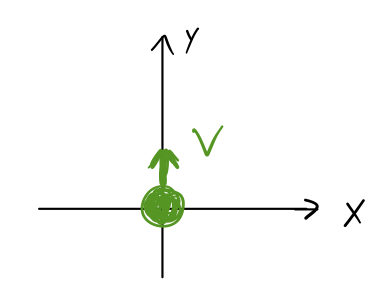
Now we'll make some simple observations. First, there are no forces and therefore no torques: since \( \vec{\Gamma} = \dot{\vec{L}} \), we conclude that \( \dot{\vec{L}} = 0 \). Moreover, the angular momentum at any moment is equal to
\[ \begin{aligned} \vec{L} = m \vec{r} \times \vec{v} \end{aligned} \]
which, since \( \vec{r} \) and \( \vec{v} \) always point along the \( y \)-axis, is always zero.
This probably seems very intuitive and trivial so far, but now what if we change coordinates?
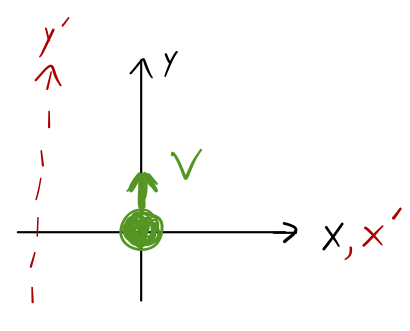
Let's call \( d \) the distance between the \( y \) and \( y' \) axes. We can evaluate \( \vec{L} \) at \( t=0 \). Then \( \vec{r} = d\hat{x}' \) and \( \vec{v} = v \hat{y}' \), so
\[ \begin{aligned} |\vec{L}| = mvd. \end{aligned} \]
Not zero! Is it changing with time? The vector \( \vec{r} \) is changing, but \( \vec{v} \) isn't, so it looks like it might be...let's evaluate later when \( y'=h \).
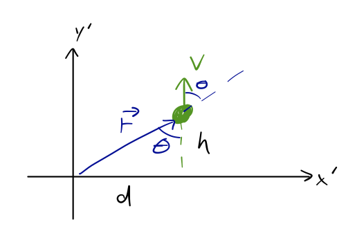
Now
\[ \begin{aligned} |\vec{L}| = mvr \sin \theta = mvd. \end{aligned} \]
Still conserved! (It should be, since there are still no torques.)
But wait, it gets better! What if I switch gravity on? In the original coordinates, we still have \( \vec{L} = 0 \) for the entire motion, because \( \vec{\Gamma} = \vec{r} \times \vec{F} \), and gravity and \( \vec{r} \) are both in the \( y \) direction. But in the primed coordinates...
\[ \begin{aligned} \vec{\Gamma} = \vec{r} \times \vec{F} = mg \vec{r} \times (-\hat{y'}) \end{aligned} \]
The angular momentum is, meanwhile,
\[ \begin{aligned} \vec{L} = m\vec{r} \times \vec{v} = m\dot{y}' \vec{r} \times \hat{y'} \end{aligned} \]
Rate of change:
\[ \begin{aligned} \dot{\vec{L}} = m\ddot{y}' (\vec{r} \times \hat{y'}) + m \dot{y}' (\dot{\vec{r}} \times \hat{y'}) \\ = m \ddot{y}' (\vec{r} \times \hat{y'}) \end{aligned} \]
since \( \dot{\vec{r}} \) always points in the \( \hat{y}' \) direction, so the second cross-product is zero. But then, we see that
\[ \begin{aligned} \vec{\Gamma} = \dot{\vec{L}} \\ (-mg) (\vec{r} \times \hat{y'}) = m\ddot{y}' (\vec{r} \times \hat{y'}) \end{aligned} \]
which is just the usual equation of motion, \( \ddot{y}' = -g \). So the motion isn't really any more complicated, but the equations certainly look more complicated in terms of angular momentum.
The main point to take away from all of this is the importance of the choice of coordinates for working with angular momentum; even seemingly general statements like "angular momentum is conserved" are strongly coordinate-dependent! This is very counter-intuitive compared to the frame dependence of linear momentum, especially since two observers who are stationary with respect to each other can disagree about angular momentum. (But they will always agree on the actual, physical motion!)
Application: Categories of rigid bodies
Previously, we noted that for any rigid object we can always find its principal axes by solving for the eigenvectors of its inertia tensor. The corresponding eigenvalues are the principal moments, equal to the diagonal entries of \( \mathbf{I} \) in the coordinates of the eigenvectors:
\[ \begin{aligned} \mathbf{I} = \left( \begin{array}{ccc} \lambda_1 & 0 & 0 \\ 0 & \lambda_2 & 0 \\ 0 & 0 & \lambda_3 \end{array} \right) \end{aligned} \]
It's useful to categorize objects based on the structure of their principal moments - we'll be able to make general statements about rotational motion in these categories.
- Spherical top: All moments equal, \( \lambda_1 = \lambda_2 = \lambda_3 \).
The cube about its CM is a spherical top, as is (obviously) the sphere. Because all three moments are equal, the eigenvectors can be chosen arbitrarily not from a plane, but from all of space; in other words, there are no unique principal axes - any direction is a principal axis.
For a spherical top, Euler's equations simply reduce to \( \lambda_i \dot{\omega_i} = 0 \). This is consistent with the idea that the principal axes aren't unique, since we already saw that for an object spinning exactly about a principal axis, the motion is absolutely stable; \( \vec{\omega} \) doesn't change.
- Symmetric top: Two moments equal, \( \lambda_1 = \lambda_2 \neq \lambda_3 \).
When I say the word "top", this is the sort of object you probably think of. The single different principal moment singles out one special axis, while the other two principal axes can be chosen freely.
Notice that when we're classifying objects like this, we must choose a pivot point as well. The cube, as we've just seen, is a spherical top when pivoting about its CM, but a symmetric top about its corner.
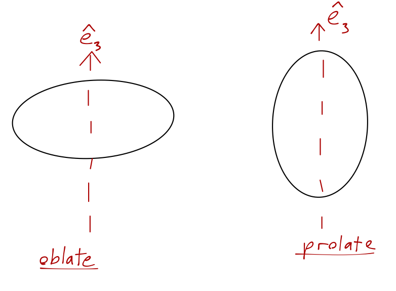
This is a good place to point out that two objects with the same principal moments will spin in exactly the same way! This is manifest in Euler's equations; the evolution of \( \vec{\omega} \) only depends on the three principal moments. So an egg spinning on its tip and a box spinning on its corner could give identical motion (if their masses and proportions are matched.)
In fact, it's sometimes useful to think about equivalent ellipsoids which will describe the same motion. In particular, the case \( \lambda_3 > \lambda_1 \) corresponds to an oblate ellipsoid, which looks squashed compared to the principal \( \hat{e}_3 \) axis. The alternative \( \lambda_3 < \lambda_1 \) is a prolate ellipsoid, which is stretched in the \( \hat{e}_3 \) direction instead.
- Linear rotor: A special symmetric top, but where \( \lambda_3 \ll \lambda_1, \lambda_2 \).
This sort of symmetric top is common in describing the energy of molecules, especially certain ones like carbon monoxide or molecular oxygen. The motion essentially reduces to considering the two-dimensional rotation about the special axis picked out by the small eigenvalue.
For example, given a pair of equal masses connected by a rigid rod, the CM is exactly centered between them. If we set up coordinates so that both masses are on the \( x \)-axis, then they both have \( y=z=0 \), and so not only do all off-diagonal elements of the tensor vanish, but also
\[ \begin{aligned} I_{xx} = m \sum_i (y_i^2 + z_i^2) = 0. \end{aligned} \]
In other words, since the masses are point particles, rotation about the axis of the rod (about \( \hat{x} \)) isn't measurable, and carries no momentum. You will encounter the linear rotor again in quantum mechanics, but we won't say much more about it here.
- Asymmetric top: All three moments unequal, \( \lambda_1 \neq \lambda_2 \neq \lambda_3 \).
This gives rise to the most complicated motion, but we can make some general statements like what we observed for stability under torque-free motion, namely that with three different principal moments \( \lambda_1 > \lambda_2 > \lambda_3 \), free rotation (about the CM, no torque) about axes \( \hat{e}_1 \) or \( \hat{e}_3 \) will be stable, while rotation about axis \( \hat{e}_2 \) is unstable.
(This observation is sometimes known as the tennis racket theorem; if you've ever played tennis, you've probably found this result out experimentally by tossing the racket up in the air and trying to catch it again. This was also the result we found for the deck of cards previously.)
Concept: Shortcuts for inertia tensors
Here we'll add a couple of simple tricks to our toolkit for calculating and/or estimating moments of inertia for certain types of objects.
Compound objects
One other important aside to note: moments of inertia for a compound object add together. This is easy to see from the definition: suppose we have a compound object that we can write as the sum of two densities, \( \rho = \rho_a + \rho_b \). Then the total moment of inertia is
\[ \begin{aligned} I_{ij} = \int dV [\rho_a + \rho_b] (r^2 \delta_{ij} - r_i r_j) = \int dV \rho_a (...) + \int dV \rho_b (...). \end{aligned} \]
So if you can split something into a small number of simple shapes, you can still easily compute its inertia tensor. The canonical example is the planet Saturn:
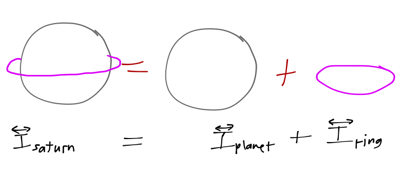
This trick works just as well with negative densities, too. For example, a hollow sphere can be treated by finding the inertia tensor for a large sphere, and subtracting the inertia tensor of a smaller sphere from it.
Exchange symmetry
Consider the general formula for the inertia tensor:
\[ \begin{aligned} I_{ij} = \int\ dV\ \rho(x,y,z) (r^2 \delta_{ij} - r_i r_j) \end{aligned} \]
For an object with uniform density, the various components are related by swapping the coordinate labels \( (x,y,z) \) with each other. For example, \( I_{xx} = r^2 - x^2 = y^2 + z^2 \), while \( I_{yy} = x^2 + z^2 \) - exchanging \( x \) with \( y \) takes one to the other.
The implication is that if an object looks the same along different directions, then some of its moments of inertia will be equal. The extreme example is a (constant density) sphere rotating about its geometric center:
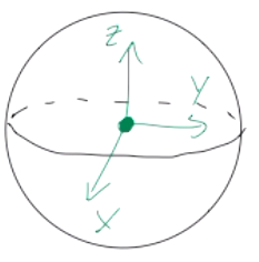
Clearly, for the sphere we can exchange any of the axis labels \( (x,y,z) \) with each other and the result will be the same. The result is that all of the sphere's moments of inertia are equal: \( I_{xx} = I_{yy} = I_{zz} \). (Thus, unsurprisingly, the sphere rotating about its center is a spherical top.)
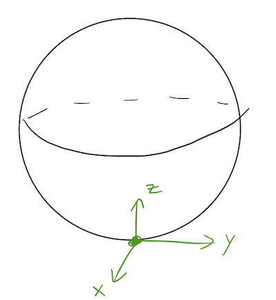
What about the inertia tensor for rotation about the a point on the edge of the sphere, instead? Now there is a clear difference between the \( z \)-direction and the other two. However, the \( x \) and \( y \) directions are clearly symmetric - we can swap one for the other and get the same geometry back. Thus, we have \( I_{xx} = I_{yy} \), but \( I_{zz} \) will be different. For this sort of rotation, a sphere is only a symmetric top.
We've only discussed diagonal moments of inertia; in this case the off-diagonal moments are all zero due to a different symmetry, reflection (which we'll talk about next.)
Because we can think of exchanging two coordinate axes with each other can be done with a rotation by \( \pi/2 \), these equalities can be thought of as arising from rotational symmetry of our object. We assumed constant density, but as long as the density of the object is also rotationally symmetric in this way, all of the observations we've made here still apply. However, exchange symmetry is a little more general; there are plenty of objects that are not invariant under an arbitrary rotation, but are under a specific rotation by \( \pi/2 \). (A cube is a good example.)
Reflection symmetry
Even for relatively complicated objects, when we calculate the inertia tensor about certain points, we will find important simplifications. Consider the general formula for the inertia tensor:
\[ \begin{aligned} I_{ij} = \int\ dV\ \rho(x,y,z) (r^2 \delta_{ij} - r_i r_j) \end{aligned} \]
Let's focus specifically on an off-diagonal component, say \( I_{xy} \):
\[ \begin{aligned} I_{xy} = - \int\ dV\ \rho(x,y,z)\ xy. \end{aligned} \]
Suppose that our object has a reflection symmetry, which means that \( \rho(-x,y,z) = \rho(x,y,z) \) and our integral is symmetric from \( -L_x \) to \( +L_x \). We can split into two equal and opposite integrals, from \( -L_x \) to \( 0 \) and \( 0 \) to \( +Lx \) - opposite because the \( x \) inside will change sign. Thus, reflection symmetry gives us \( I{xy} = 0 \) - no matter how complicated the object's geometry or density are!
Now, there are three off-diagonal moments; reflection symmetry in one direction will get rid of two of them (it should be obvious that \( I_{xz} = 0 \) as well in our example above.) If our object has reflection symmetry about any two axes, then all three off-diagonal moments will vanish.
Let's try this with a relatively complicated object that you don't want to directly calculate \( \mathbf{I} \) for: a tennis racket.
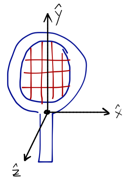
There is one obvious reflection symmetry from the diagram: reflection in the \( x \)-direction. This will eliminate \( I_{xy} \) and \( I_{xz} \) immediately. Although it's less obvious from the diagram, the tennis racket has the same shape along the \( z \)-axis, which means it is also symmetric under reflection in \( z \). This eliminates the remaining off-diagonal moment \( I_{yz} \), leaving a diagonal inertia tensor:
\[\mathbf{I}_{\rm racket} = \left(\begin{array}{ccc} I_{1} & 0 & 0 \\ ...&I_{2}&0 \\ ...&...&I_{3} \end{array} \right)\]
The racket is definitely not symmetric along the \( y \)-axis, of course, but the point is that it doesn't matter - we only need two out of three reflection symmetries to eliminate all off-diagonal moments (and skip having to calculate them explicitly, or work out eigenvectors.)
Once we know that the inertia tensor is diagonal, as we discussed last time, the size of the moments of inertia will be proportional to the cross-sectional area of the object along each axis:
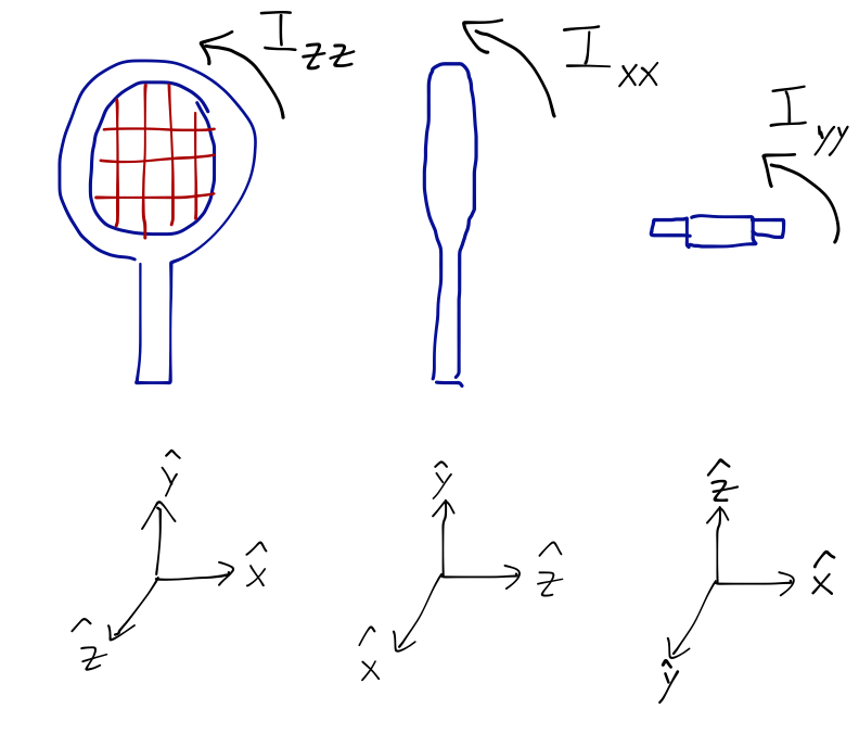
Clearly we have \( I_{zz} > I_{xx} > I_{yy} \), so the racket is an asymmetric top as expected. Moreover, we can see that motion around the \( x \)-axis will be unstable and exhibit tumbling.
Concept: Laminar objects
An interesting class of objects are laminar objects, which are objects with almost no thickness in one direction, for example a flat and very thin sheet of metal. All of our formulas so far have been three-dimensional, so it's not so obvious what to do when one dimension nearly vanishes.
Suppose we take the \( z \)-direction to be the one along which our object is very thin. Let's think about the total mass of the object first:
\[ \begin{aligned} M = \int dV \rho(x,y,z) = \int_{-\epsilon}^{\epsilon} dz \int dA \rho(x,y,z), \end{aligned} \]
where \( dA = dx dy \). Suppose that we do the area integral first, which leaves us with
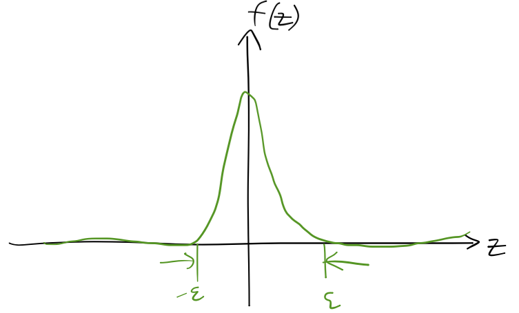
\[ \begin{aligned} M = \int_{-\epsilon}^{\epsilon} dz\ f(z). \end{aligned} \]
Whatever the function \( f(z) \) looks like, we know that the total mass \( M \) has to be finite as \( \epsilon \rightarrow 0 \). But this means that as we make \( \epsilon \) smaller and smaller, more of the area under the function \( f(z) \) has to be accumulating in a tiny region around \( z=0 \):
The limit of this squeezing as \( \epsilon \rightarrow 0 \) actually gives us a special function known as the Dirac delta function, \( \delta(z) \). The delta function is equal to zero everywhere except \( z=0 \), where it's infinite. This may not seem perfectly well-defined to you (and technically, it's not even a function but a "distribution"), but as long as it's inside an integral, we will find sensible results. In particular, the Dirac delta function obeys the equation
\[ \begin{aligned} \int_{-\infty}^\infty dz\ f(z) \delta(z-a) = f(a). \end{aligned} \]
So you can think of the delta function as an object which picks out a certain value of a function from underneath an integral. We have to be integrating over the region with the delta-function spike for this to work; if we integrate from \( -1 \) to \( 1 \) over \( \delta(z-2) \), for example, then we'll just get zero.
We can thus write the density of our infinitesmally thin laminar object as
\[ \begin{aligned} \rho(x,y,z) = \sigma(x,y) \delta(z), \end{aligned} \]
assuming the pivot point is at \( z=0 \); this guarantees that we get a finite total mass, no matter what \( \sigma(x,y) \) looks like. Here \( \sigma \) is standard notation for an area mass density, with units of mass/length \( ^2 \).
Notice, by the way, that the delta functions all have inverse units of whatever is inside them, in this case length. You can see this by noticing that
\[ \begin{aligned} \int dx\ \delta(x) = 1, \end{aligned} \]
where the units on the left-hand side are length (\( dx \)) and 1/length (\( \delta(x) \)).
There's one immediate simplification that happens for a laminar object: any off-diagonal moments involving the direction perpendicular to the flat surface are zero. For example, in our example using the \( z \)-axis, we see that
\[ \begin{aligned} I_{xz} = \int\ dV\ \sigma(x,y) \delta(z)\ xz \end{aligned} \]
and the \( z \)-integral just gives us zero. Similarly, \( I_{yz} = 0 \). However, we're not guaranteed that we have a symmetric top: as long as the area density \( \sigma(x,y) \) is not constant, in general we will find three different diagonal moments of inertia. The one general statement we can make is that the axis perpendicular to the plane of the lamina is always a principal axis, because of the vanishing off-diagonal components.
Application: Free rotation of a symmetric top
Back to Euler's equations with no torques:
\[ \begin{aligned} \lambda_1 \dot{\omega_1} - (\lambda_2 - \lambda_3) \omega_2 \omega_3 = 0 \\ \lambda_2 \dot{\omega_2} - (\lambda_3 - \lambda_1) \omega_3 \omega_1 = 0 \\ \lambda_3 \dot{\omega_3} - (\lambda_1 - \lambda_2) \omega_1 \omega_2 = 0. \end{aligned} \]
Last time, we categorized different kinds of rigid bodies into asymmetric, symmetric, and spherical tops, based on how many equal principal moments of inertia they had. As far as motion, we already covered the spherical top: it will stably rotate about any axis at all. We've done what we can with the asymmetric top for now, so let's move on to the symmetric top.
We'll choose \( \lambda_3 \) to be the unique eigenvalue of our symmetric top, so that \( \lambda_1 = \lambda_2 \). Then only the last equation simplifies,
\[ \begin{aligned} \lambda_3 \dot{\omega}_3 = 0. \end{aligned} \]
So once again, we find a certain amount of stability if \( \Gamma_3 = 0 \): \( \dot{\omega}_3 = 0 \). However, \( \omega_1 \) and \( \omega_2 \) can still evolve in time if they are non-zero. For the asymmetric top, we could only study the case where \( \omega_1 \) and \( \omega_2 \) were very small; we explored the stability of rotation mostly around the \( \omega_3 \) axis. Now we can go a bit further!
We can reorganize the other two equations, plugging in \( \lambda_1 \) for \( \lambda_2 \):
\[ \begin{aligned} \dot{\omega}_1 = \frac{(\lambda_1 - \lambda_3) \omega_3}{\lambda_1} \omega_2 = \Omega_b \omega_2 \\ \dot{\omega}_2 = -\frac{(\lambda_1 - \lambda_3) \omega_3}{\lambda_1} \omega_1 = -\Omega_b \omega_1, \end{aligned} \]
defining the body precession frequency
\[ \begin{aligned} \Omega_b = \frac{\lambda_1 - \lambda_3}{\lambda_1} \omega_3. \end{aligned} \]
This is a coupled set of differential equations, which we haven't learned how to solve in general yet. But we can use the trick you learned last semester, and used on the homework for rotating frames: we define the complex variable
\[ \begin{aligned} \eta \equiv \omega_1 + i \omega_2. \end{aligned} \]
Notice that if we add \( i \) times the second equation to the first, we have
\[ \begin{aligned} \dot{\omega_1} + i \dot{\omega_2} = \Omega_b (\omega_2 - i\omega_1) \\ = -i \Omega_b (\omega_1 + i \omega_2), \end{aligned} \]
so we can combine both differential equations into
\[ \begin{aligned} \dot{\eta} = -i \Omega_b \eta. \end{aligned} \]
We know the solution to this is just an exponential,
\[ \begin{aligned} \eta(t) = \eta_0 e^{-i \Omega_b t}. \end{aligned} \]
Setting \( \eta_0 = \omega_0 + 0i \) to put the initial \( \omega_2 = 0 \), we take the real and imaginary part of \( \eta \) to get back \( \omega_1 \) and \( \omega_2 \):
\[ \begin{aligned} \vec{\omega} = (\omega_0 \cos (\Omega_b t), -\omega_0 \sin (\Omega_b t), \omega_3). \end{aligned} \]
So \( \omega_3 \) remains constant, while \( \omega_1 \) and \( \omega_2 \) rotate around at frequency \( \Omega_b \).
This motion - constant and periodic rotation of the vector \( \vec{\omega} \) about a symmetry axis - is called precession (hence our name for \( \Omega_b \).) Notice that in this frame,
\[ \begin{aligned} \frac{d\vec{\omega}}{dt} = (-\Omega_b \omega_0 \sin (\Omega_b t), -\Omega_b \omega_0 \cos (\Omega_b t), 0) \\ = (0, 0, \Omega_b) \times (\omega_0 \cos (\Omega_b t), -\omega_0 \sin (\Omega_b t), \omega_3) \\ = \vec{\Omega_b} \times \vec{\omega} \end{aligned} \]
which is just the familiar vector equation telling us that \( \vec{\omega} \) rotates about the axis of \( \vec{\Omega_b} = \Omega_b \hat{e}_3 \) at constant angular velocity \( \Omega_b \).
Notice that the sign of \( \Omega_b \) can change, depending on the values of the principal moments. If the unique moment \( \lambda_3 \) is the smallest moment, then we have a prolate symmetric top; otherwise, the top is said to be oblate if \( \lambda_3 \) is larger. The precession direction is opposite in these two cases (counter-clockwise about \( \hat{e}_3 \) for a prolate top, from the right-hand rule.)
There's a more geometrical way to look at this, based on conservation laws. In the body frame, notice that our solution gives a constant magnitude for the angular velocity vector:
\[ \begin{aligned} |\vec{\omega}| = \sqrt{\omega_0^2 \cos^2 (\Omega_b t) + \omega_0^2 \sin^2 (\Omega_b t) + \omega_3^2} = \textrm{const} \end{aligned} \]
If we sketch the motion of the vector, it traces out a cone, sometimes called the body cone:
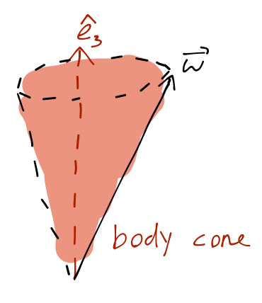
The same is true for the angular momentum \( \vec{L} \), although it points in a slightly different direction from \( \vec{\omega} \) so it won't trace out the same cone.
What about in the space frame? We know that because there are no torques \( \vec{L} \) is constant, and the total energy \( T = \frac{1}{2} \vec{\omega} \cdot \vec{L} \) is constant too. So the component of \( \vec{\omega} \) pointing along \( \vec{L} \) is constant. With the magnitude of \( \vec{\omega} \) fixed, the only possible motion is precession once again, this time tracing out the space cone:
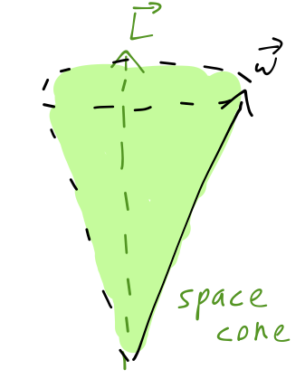
If we imagine the motion of \( \vec{\omega} \) and \( \hat{e}_3 \) in the space frame, then \( \vec{\omega} \) is the point of contact between the body and space cones, and we can picture the imaginary body cone rolling around the (also imaginary) space cone without slipping.
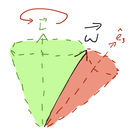
It's much more informative to see this in motion instead of my still sketches:
YouTube - free precession of a simulated satellite
If you watch very carefully and compare the angular momentum vector to the solar panels on the satellite, you should be able to see that the direction of \( \vec{\omega} \) is changing in the body frame (obviously it's changing in the space frame, which is our point of view.)
This leads us to yet another interesting effect involving the rotation of the Earth. Because the Earth does have a slight bulge at the center, it doesn't quite spin as a spherical top, but is better described as a symmetric top! This means that independent of any torques, it will undergo the free precession that we just described here. As a reminder, the precession frequency is
\[ \begin{aligned} \Omega_b = \frac{\lambda_1 - \lambda_3}{\lambda_1} \omega_3 \end{aligned} \]
and the Earth's moment about the pole \( \lambda_3 \) is about \( 1/300 \) larger than the other moment, \( \lambda_1 \). This gives a precession frequency of
\[ \begin{aligned} \Omega_b = \omega_3 / 300 \end{aligned} \]
or about 300 days for a full cycle. The amplitude is much harder to predict, of course, since it depends on the misalignment between the Earth's rotational and polar symmetry axes. In fact, this small wobble in the Earth's rotation was predicted by both Newton and Euler over 200 years ago, but wasn't discovered until 1891, by American astronomer Seth Chandler; it is called the Chandler wobble after him.
It's an interesting lesson in physics, because part of the reason that Chandler finally found the wobble is because he didn't trust the theory completely! Most previous searches had been narrowly focused on fluctuations with period of about 300 days, but Chandler looked more broadly and finally found the predicted rotation with a period of over 400 days. The difference is mainly explained by the fact that the Earth is not quite a rigid body.
Even more interesting, the Chandler wobble is not precisely fixed; its amplitude fluctuates somewhat over time. Oddly, the phase of the Chandler wobble has occasionally changed quickly and dramatically, definitively in 1925 and (according to recent observations) again around 1850 and 2005. It remains an open problem in geophysics to explain what effect could cause the wobble to suddenly change in such a way!
Concept: Rotation matrices
To make progress into more complicated and interesting problems, we need to understand how to describe rotations of coordinates in general. First, we need to talk in general about coordinate transformations.
If you and I come across a ladder leaning against the wall, let's say I use the floor and wall as my \( x-y \) coordinates, and I measure the distances under the ladder on the floor and wall in yards. On the other hand, you decide the direction of the ladder is a better coordinate, and just measure its length directly, in meters. Our numbers will be different, we will have different ideas about the size of the components of the vector describing the ladder; but once we account for units, we must agree on its length, and on the angle it makes with the wall and the floor, and so forth.
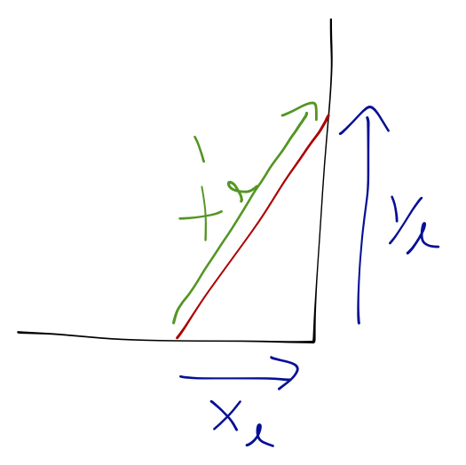
Here we are taking the point of view here that the vector \( \vec{v} \), or the ladder, is fixed in space, and we're rotating our coordinate system around it. This is called a passive transformation. On the other hand, we could sit in a fixed coordinate system and actually change the orientation of the vector, for example if I start with the ladder oriented straight up and then lean it against the wall; this is an active transformation.
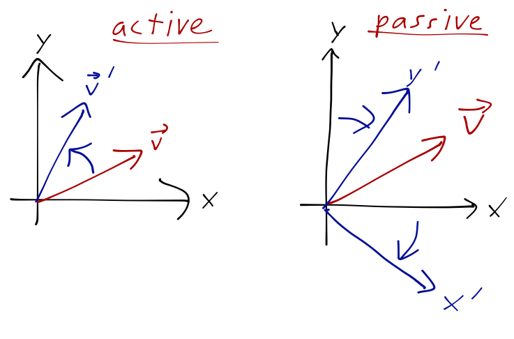
In physics terms, the difference is in whether the object is moving, or the observer looking at it is. The mathematics of these sorts of transformations, for e.g. rotations, are very similar but with crucial minus signs; a vector rotating clockwise looks just like a coordinate rotation counter-clockwise. So be careful with formulas you get from other sources like Wikipedia! You can always just ask what happens with the formula in front of you if you rotate by something like \( \pi/2 \) or \( \pi \), and see that the result is what you expect.
Let's consider a passive rotation from coordinates \( (x,y,z) \) to \( (x',y',z') \), as pictured. In the original (un-primed) frame, we can divide the vector \( \vec{v} \) into components,
\[ \begin{aligned} \vec{v} = {v}_x \hat{x} + {v}_y \hat{y} + {v}_z \hat{z}. \end{aligned} \]
Of course, we can do the same thing in the primed coordinates,
\[ \begin{aligned} \vec{v} = {v}_{x'} \hat{x}' + {v}_{y'} \hat{y}' + {v}_{z'} \hat{z}'. \end{aligned} \]
Any differences between the components of \( \vec{v} \) in the two coordinate systems is because the unit vectors themselves are different. We can write this out in terms of dot products between the unit vectors,
\[ \begin{aligned} v_{x'} = \vec{v} \cdot \hat{x}' \\ = (v_x \hat{x} + v_y \hat{y} + v_z \hat{z}) \cdot \hat{x}' \\ = v_x (\hat{x} \cdot \hat{x}') + v_y (\hat{y} \cdot \hat{x}') + v_z (\hat{z} \cdot \hat{x}'). \end{aligned} \]
Note that it doesn't matter whether we think of \( \hat{x}' \) as a vector in the unprimed coordinates, or vice-versa; the dot products are all the same. If we expand all three components of \( \vec{v} \) in the same way, we find a matrix equation
\[ \begin{aligned} \left(\begin{array}{c} v_{x'} \\ v_{y'} \\ v_{z'} \end{array} \right) = \left( \begin{array}{ccc} \hat{x} \cdot \hat{x}' & \hat{y} \cdot \hat{x}' & \hat{z} \cdot \hat{x}' \\ \hat{x} \cdot \hat{y}' & \hat{y} \cdot \hat{y}' & \hat{z} \cdot \hat{y}' \\ \hat{x} \cdot \hat{z}' & \hat{y} \cdot \hat{z}' & \hat{z} \cdot \hat{z}' \end{array} \right) \left( \begin{array}{c} v_x \\ v_y \\ v_z \end{array} \right) \end{aligned} \]
or more compactly
Transformation of vectors under rotation
\[ \begin{aligned} \vec{v}' = \mathbf{R} \vec{v}. \end{aligned} \]
\( \mathbf{R} \) is a rotation matrix, which transforms the vector \( \vec{v} \) from the unprimed to the primed coordinates. (Remember that we're taking the attitude that this is a passive transformation, so \( \vec{v} \) is the same vector; I'm just writing \( \vec{v}' \) as shorthand for "the vector \( \vec{v} \) expressed in the primed coordinates.")
What if we wanted to go back the other way, and find the components of a vector in the unprimed coordinates from the primed ones? We can write that as a matrix of dot products again, for example the \( \hat{x} \) component will be
\[ \begin{aligned} \vec{v} \cdot \hat{x} = (v_{x'} \hat{x}' + v_{y'} \hat{y}' + v_{z'} \hat{z}') \cdot \hat{x} \end{aligned} \]
and we end up with another rotation matrix, which I can write as \( \vec{v} = \mathbf{R'} \vec{v}' \). How is \( \mathbf{R'} \) related to \( \mathbf{R} \)? Since the order in dot-products doesn't matter, you can check that it's clearly the transpose matrix:
\[ \begin{aligned} \mathbf{R'} = \mathbf{R}^T. \end{aligned} \]
Of course, since applying \( \mathbf{R} \) and then \( \mathbf{R}' \) takes us from unprimed to primed coordinates and then back again, we also know that
\[ \begin{aligned} \mathbf{R'} \mathbf{R} = \mathbf{R}^T \mathbf{R} =\mathbf{1}. \end{aligned} \]
A matrix whose transpose is also its inverse is known as an orthogonal matrix; all rotation matrices are orthogonal, as we can now see.
As I've repeatedly warned, the inertia tensor \( \mathbf{I} \) is intimately connected to the choice of coordinates, which certainly means that a rotation will change its form. But how is \( \mathbf{I'} \) related to \( \mathbf{I} \)? We know that the relationship between \( \vec{L} \) and \( \vec{\omega} \) should still be the same after rotation:
\[ \begin{aligned} \vec{L'} = \mathbf{I'} \vec{\omega'}. \end{aligned} \]
But we can write the primed vectors using the rotation matrix:
\[ \begin{aligned} \mathbf{R} \vec{L} = \mathbf{I'} \mathbf{R} \vec{\omega}. \end{aligned} \]
Multiply on the left by \( \mathbf{R}^T \):
\[ \begin{aligned} \mathbf{R}^T \mathbf{R} \vec{L} = \mathbf{R}^T \mathbf{I'} \mathbf{R} \vec{\omega} \\ \vec{L} = (\mathbf{R}^T \mathbf{I'} \mathbf{R}) \vec{\omega}, \end{aligned} \]
since as we just saw, \( \mathbf{R}^T \) is the inverse of \( \mathbf{R} \). But now, the matrix in the middle is just the original \( \mathbf{I} \)! Multiplying by \( \mathbf{R} \) and \( \mathbf{R}^T \) again to move things around, we see that
Transformation of the inertia tensor under rotation
\[ \begin{aligned} \mathbf{I'} = \mathbf{R} \mathbf{I} \mathbf{R}^T. \end{aligned} \]
Now we can see in detail what I meant when I said that "a tensor is a matrix that transforms in a certain way under coordinate changes." In fact, this equation is sometimes presented as the definition of a tensor. So we've seen three kinds of transformations under a rotation:
\[ \begin{aligned} \vec{v'} \cdot \vec{w'} = \vec{v} \cdot \vec{w} \\ \vec{v'} = \mathbf{R} \vec{v} \\ \mathbf{I'} = \mathbf{R} \mathbf{I} \mathbf{R}^T \end{aligned} \]
describing, in turn, a scalar, a vector, and a tensor. It's instructive to write these out again in index notation:
\[ \begin{aligned} \sum_i v'_i w'_i = \sum_i v_i w_i \\ v'_i = \sum_j R_{ij} v_j \\ I'_{ij} = \sum_{k,l} R_{ik}^T I_{kl} R_{lj} \\ = \sum_{kl} I_{kl} R_{ki} R_{lj} \end{aligned} \]
There is, in fact, a very simple pattern here. For any object with any number of indices that aren't already being summed over, under a rotation, that index is "contracted" (summed over with a common index) with one copy of the rotation matrix. In other words, we can imagine an arbitrarily complicated, higher-dimensional tensor, and we know how it transforms under rotation:
\[ \begin{aligned} T_{ijkl...} = \sum_{abcd} T_{abcd...} R_{ai} R_{bj} R_{ck} R_{dl} ... \end{aligned} \]
In classical mechanics, we'll never go any further than a matrix, so you don't have to worry about these more abstract tensor structures. If you go on to study general relativity, you will encounter them there!