Concept: Functions of matrices
Everything we went through in terms of solving the coupled oscillator problem with normal modes as a generalized eigenvalue problem works, but it's a little arcane; there are a lot of steps and new terms, and we had to make an educated guess halfway through.
There's a much more direct way to get the answer, which should help to clarify why the normal mode approach actually works. But to understand the direct approach, we need to take a detour into some math, to define how to take functions of matrices.
We've seen before how to define basic operations on matrices, including powers; the matrix \( A^n \) is just obtained by multiplying \( A \) together, \( n \) times. We can make use of this to define matrix functions in terms of their power series. For example, the exponential of a matrix is defined to be:
\[ \begin{aligned} \exp(A) = \sum_{n=0}^{\infty} \frac{1}{n!} A^n. \end{aligned} \]
In principle, this series always converges, so we can always define the exponential of a matrix in this way. In practice, it's an infinite series, so we can only find an explicit answer when there is some repeating pattern in the powers of \( A \) (or if \( A^m = 0 \) for some \( m \), which terminates the series.) For example, let's try
\[ \begin{aligned} A = \left(\begin{array}{cc} 1&2 \\ 0&1 \end{array}\right). \end{aligned} \]
The first few powers are easy to compute:
\[ \begin{aligned} A^2 = \left(\begin{array}{cc} 1&4 \\ 0&1 \end{array} \right) \\ A^3 = \left(\begin{array}{cc} 1&6 \\ 0&1 \end{array} \right) \\ (...)\\ A^n = \left(\begin{array}{cc} 1&2n \\ 0&1 \end{array} \right) \end{aligned} \]
So we can rewrite the infinite sum as
\[ \begin{aligned} \exp(\mathbf{A}) = \sum_{n=0}^\infty \frac{1}{n!} \left( \begin{array}{cc} 1& 2n \\ 0 & 1 \end{array} \right). \end{aligned} \]
We can evaluate the sum inside each entry of the matrix separately:
\[ \begin{aligned} \sum_{n=0}^\infty \frac{1}{n!} = e, \\ \sum_{n=0}^\infty \frac{2n}{n!} = 2\sum_{n=0}^\infty \frac{1}{(n-1)!} = 2\sum_{m=0}^\infty \frac{1}{m!} = 2e, \end{aligned} \]
giving the result
\[ \begin{aligned} \exp(\mathbf{A}) = \left( \begin{array}{cc} e & 2e \\ 0 & e \end{array} \right) \end{aligned} \]
Note that this is not the same as just taking the exponential of the individual elements of the matrix! (That would have given us \( e^2 \) in the corner, and \( 1 \) in the other corner, both of which are wrong.)
Of course, not every matrix is guaranteed to have a nice, recurring expression for \( A^n \) that we can sum up like this. But there's one other class of matrices that's particularly easy to exponentiate, which are the diagonal matrices. Since for an \( m \times m \) diagonal matrix,
\[ \begin{aligned} \mathbf{A} = \left(\begin{array}{cccc} a_1 &&&\\ &a_2&& \\ &&...& \\ &&&a_m \end{array} \right) \Rightarrow \mathbf{A}^n = \left(\begin{array}{cccc} a_1^n &&&\\ &a_2^n&& \\ &&...& \\ &&&a_m^n \end{array} \right) \end{aligned} \]
we can do the sum no matter what the components are:
\[ \begin{aligned} \exp(\mathbf{A}) = \left(\begin{array}{cccc} e^{a_1} &&&\\ &e^{a_2}&& \\ &&...& \\ &&&e^{a_n} \end{array} \right) \end{aligned} \]
Other functions can also be defined as power series, but we have to be careful about the existence of the result in general. Square root is a much trickier function. Certainly, we can define \( B \) to be the matrix square-root of \( A \) as long as it satisfies the equation
\[ \begin{aligned} B^2 = A. \end{aligned} \]
But writing this as a function isn't particularly nice; for one thing, there is often not a unique solution to this equation; many matrices can be square roots for a given \( A \). (The humble 2x2 identity matrix has an infinite number of square roots! Most 2x2 matrices have four.) Neither is existence of a solution guaranteed; there are some matrices with no square root.
The first piece of good news is that if \( A \) is diagonal, then its square root is both unique and easy to find:
\[ \begin{aligned} \sqrt{ \mathbf{A}} = \left(\begin{array}{cccc} \sqrt{a_1} &&&\\ &\sqrt{a_2}&& \\ &&...& \\ &&&\sqrt{a_n} \end{array} \right) \end{aligned} \]
(Notice that this matrix isn't quite unique; we could have put minus signs into any of the diagonal entries, and it would still square to \( A \). But like the square-root symbol, we take the positive root by convention. The square root matrix with all positive eigenvalues is sometimes called the principal square root.)
Of course, most matrices aren't diagonal. But as long as the matrix is diagonalizable, i.e. as long as there exists a coordinate change which we can apply to make it diagonal, then we can always find the square root (or other functions) in this way. You'll recall this was true for the inertia tensor, working in the principal axes - coordinates given by the eigenvectors. The same will be true for the coupled oscillator problem, because the matrices \( \mathbf{M} \) and \( \mathbf{K} \) are both real and symmetric.
Formula: General solution for the coupled oscillator
Our starting point is again the system of differential equations of motion, written as a matrix equation:
\[ \begin{aligned} M \ddot{\vec{x}} = -K \vec{x}. \end{aligned} \]
What if we just try to solve this like the ordinary simple harmonic oscillator? First, we "divide out" the mass, by multiplying on the left by \( M^{-1} \):
\[ \begin{aligned} \ddot{\vec{x}} = -(M^{-1} K) \vec{x} \end{aligned} \]
Now, as a reminder, one way to write the solution to the scalar SHO is by using a complex exponential:
\[ \begin{aligned} x(t) = A e^{i\omega t} \Rightarrow \ddot{x} = -\omega^2 A e^{i\omega t} = -\omega^2 x. \end{aligned} \]
The complex number is a convenience, of course; the position of a cart \( x(t) \) is still a real number. By taking the real part, or careful choices of the (possibly complex) coefficient \( A \), we can make sure we get a real \( x(t) \) in the end. I'm just using the complex notation because it'll make the following explanation easier, but we could just write sine/cosine too.
So, why don't we just do the same thing for our matrix equation? If
\[ \begin{aligned} \vec{x}(t) = e^{\pm i \sqrt{M^{-1} K} t} \vec{A} \end{aligned} \]
then
\[ \begin{aligned} \ddot{\vec{x}}(t) = - (M^{-1} K) \vec{x} \end{aligned} \]
and we can immediately see that the most general possible solution to the equation is just given by adding these two solutions up:
\[ \begin{aligned} \vec{x}(t) = e^{i\sqrt{M^{-1} K} t} \vec{x}_+ + e^{-i\sqrt{M^{-1} K} t} \vec{x}_- \end{aligned} \]
where \( \vec{x}+, \vec{x}- \) are determined by the 2N initial conditions as usual (starting position and speed of each mass, say.)
To take these functions of our matrix \( M^{-1} K \), we have to diagonalize it, which means we just need to find its eigenvalues and eigenvectors:
\[ \begin{aligned} (M^{-1} K - \lambda_i \mathbf{1}) \vec{v}_i = 0 \end{aligned} \]
and the eigenvalue equation is
\[ \begin{aligned} \det(M^{-1} K - \lambda \mathbf{1}) = \det(M) \det(K - \lambda M) = 0. \end{aligned} \]
This gives us back what I called the "generalized eigenvalue equation" last time; now you can really see that this is just the normal eigenvalue equation, but for the more complicated matrix \( M^{-1} K \)! (We know \( \det{M} \neq 0 \), so don't worry about that term.) Because the combined matrix \( M^{-1} K \) is still real and symmetric, like the inertia tensor we are guaranteed to be able to diagonalize in any problem.
In a coordinate system defined by the eigenvectors of this matrix, we know that e.g. in the 2x2 case
\[ \begin{aligned} M^{-1} K \rightarrow \left( \begin{array}{cc} \lambda_1 & 0 \\ 0 & \lambda_2 \end{array} \right) = \left( \begin{array}{cc} \omega_1^2 & 0 \\ 0 & \omega_2^2 \end{array} \right), \end{aligned} \]
and our solution becomes simply
\[ \begin{aligned} \vec{x}(t) = \left( \begin{array}{cc} e^{i\omega_1 t} & 0 \\ 0 & e^{i\omega_2 t} \end{array} \right) \vec{x}_+ + \left( \begin{array}{cc} e^{-i\omega_1 t} & 0 \\ 0 & e^{-i\omega_2 t} \end{array} \right) \vec{x}_-, \end{aligned} \]
where \( \vec{x}+ \) and \( \vec{x}- \) are constants determined by the initial conditions of our problem. It's vital to remember that we've changed coordinates here, to what are known as the normal coordinates, \( \xi_i \). As usual, we can expand any vector in components of either coordinate system:
\[ \begin{aligned} \vec{x} = x \hat{x} + y \hat{y} = \xi_1 \hat{\xi}_1 + \xi_2 \hat{\xi}_2. \end{aligned} \]
So to quickly recap, here's the formula for solving coupled oscillator problems:
- Find the equations of motion, i.e. solve for the acclerations \( \ddot{\vec{x}} \). Make sure to expand around equilibrium, so \( \ddot{\vec{x}} = 0 \) if \( \vec{x}=0 \).
- Write the equations in the form \( \mathbf{M} \ddot{\vec{x}} = -\mathbf{K} \vec{x} \).
- Solve the generalized eigenvalue equation \( \det(\mathbf{K} - \omega^2 \mathbf{M}) = 0 \) for the normal frequencies, \( \omega_i \).
- Solve the generalized eigenvector equation \( (\mathbf{K} - \omega_i^2 \mathbf{M})\vec{\xi}_i = 0 \) for the normal modes, \( \vec{\xi}_i \).
- The general solution is then
\[ \begin{aligned} \vec{x}(t) = \sum_i \vec{\xi}_i A_i \cos (\omega_i t - \delta_i), \end{aligned} \]
where initial conditions will determine \( A_i \) and \( \delta_i \).
As we've just investigated, all of this is equivalent to simply stating that the general solution is
\[ \begin{aligned} \vec{x}(t) = \exp \left(\pm i \sqrt{\mathbf{M}^{-1} \mathbf{K}} t \right) \vec{A} \end{aligned} \]
and then diagonalizing the matrix \( \mathbf{M}^{-1} \mathbf{K} \) in order to evaluate the exponential and square-root functions. Once again, diagonalization is at the center of what we're doing here, just as it was for the inertia tensor, which is why we rely on the same eigenvalue/eigenvector procedure to find our "clever choice of coordinates". There's sort of a mental map you can remember between inertia tensors and coupled oscillators, in fact:
- Normal coordinates \( \leftrightarrow \) body-frame coordinates
- Normal frequencies \( \leftrightarrow \) principal moments
- Normal modes \( \leftrightarrow \) principal axes
Application: Expansion at equilibrium
Our study of coupled oscillators is much more general than it might seem. In fact, a huge number of physical processes can be reduced to a coupled harmonic oscillator description. Michael Peskin (a famous particle physicist) goes so far as to define physics as "that subset of human experience that can be reduced to coupled harmonic oscillators".
The ubiquitous nature of the coupled SHO isn't mysterious; it comes from the fact that we are often interested in small changes of a system around some equilibrium. Suppose we have just written down the Lagrangian and wrote out the equations of motion for some physical process. If we gather all of the accelerations on one side, we can almost always write the equations of motion in the form
\[ \begin{aligned} \ddot{q_i} = f_i(q_1, q_2, ..., q_n) \end{aligned} \]
for a system with \( n \) degrees of freedom. Now assume that we've located an equilibrium point, \( {Q_i} \), for which the system will remain at rest, i.e.
\[ \begin{aligned} f_i(Q_1, Q_2, ..., Q_n) = 0. \end{aligned} \]
We can consider small perturbations of the system around the (constant) equilbrium point:
\[ \begin{aligned} q_i(t) = Q_i + \eta_i(t) \end{aligned} \]
where the \( \eta_i \) are all small numbers. Without knowing anything at all about the functions \( f_i \), we can deal with these small perturbations by Taylor expanding:
\[ \begin{aligned} f(q_1, q_2, ..., q_n) = f(Q_1, Q_2, ..., Q_n) + \sum_{j=1}^{n} \left.\frac{\partial f_i}{\partial q_j}\right|_{q=Q} (q_j - Q_j) + ... \\ = \sum_{j=1}^n \left.\frac{\partial f_i}{\partial q_j}\right|_{q=Q} \eta_j + ... \end{aligned} \]
Since (in our expansion) \( \ddot{q_i} = \ddot{\eta_i} \), after the Taylor expansion our equations of motion become
\[ \begin{aligned} \ddot{\eta}_i = \sum_{j=1}^n \left.\frac{\partial f_i}{\partial q_j}\right|_{q=Q} \eta_j \end{aligned} \]
This can be re-written as a matrix equation,
\[ \begin{aligned} \ddot{\vec{\eta}} = \mathbf{F} \vec{\eta}. \end{aligned} \]
So any physical system close enough to equilibrium will behave as a simple harmonic oscillator! This is exactly the equation we've been studying for the masses and springs; for that particular system we identify \( \mathbf{F} = -\mathbf{M}^{-1} \mathbf{K} \). As always, the general solution is
\[ \begin{aligned} \eta_i(t) = \sum_i \vec{v}_i \left[ A_i e^{\sqrt{\lambda_i} t} + B_i e^{-\sqrt{\lambda_i} t} \right], \end{aligned} \]
where \( \lambda_i \) and \( \vec{v}_i \) are the eigenvalues and eigenvectors of \( \mathbf{F} \).
In the case of the masses and springs, the eigenvalues of \( F \) were all negative (because \( M^{-1} K \) has all positive eigenvalues), so the only solution was simple harmonic motion - sines and cosines with angular frequency \( \sqrt{\lambda} \). More generally, not every equilibrium point is totally stable; sometimes the equilibrium is unstable, and the time-dependence is exponential instead of oscillating.
Of course, a concern with a completely general \( \mathbf{F} \) is that it will not necessarily be real and symmetric - something we relied upon to ensure that we can find a full set of eigenvectors and eigenvalues in order to write this solution down. In the most general case, this is not guaranteed. However, we can easily see that for any system described by a Lagrangian, \( \mathbf{F} \) is indeed real and symmetric. We can write the most general possible Lagrangian in the form
\[ \begin{aligned} \mathcal{L} = \frac{1}{2} \sum_{i,j} T_{ij}(q_1, q_2, ..., q_n) \dot{q}_i \dot{q}_j - V(q_1, q_2, ..., q_n), \end{aligned} \]
where \( T_{ij} \) is a symmetric tensor that can also depend on coordinates. (A simple example we've seen before is given by the kinetic terms in spherical coordinates.) Now, the Euler-Lagrange equations take the form
\[ \begin{aligned} \frac{d}{dt} \left( \frac{\partial \mathcal{L}}{\partial \dot{q_i}} \right) = \frac{\partial \mathcal{L}}{\partial q_i} \end{aligned} \]
This will be messy if we write it out in general, but if we appeal to our equilibrium expansion \( q_i(t) = Q_i + \eta_i(t) \) once more and keep only terms at first order in \( \eta \), then we find:
\[ \begin{aligned} \sum_j T_{ij}(Q_1, ..., Q_n) \ddot{\eta}_j = - \sum_j \left.\frac{\partial^2 V}{\partial q_i \partial q_j}\right|_{q=Q} \eta_j \end{aligned} \]
or as a matrix equation treating \( \eta_j \) as a vector,
\[ \begin{aligned} \mathbf{T} \ddot{\vec{\eta}} = -\mathbf{V}'' \vec{\eta}. \end{aligned} \]
So the matrix \( \vec{F} \) above is exactly \( -\mathbf{T}^{-1} \mathbf{V}'' \), and because transposing \( \mathbf{V}'' \) just swaps the order of \( q_i \) and \( q_j \) in the partial second derivative, we see that for any physical system described by a Lagrangian, expansion in coupled oscillators always gives a real, symmetric \( \mathbf{F} \) matrix and we can always use our eigenvector technique to solve.
(This is glossing over some details - the full proof by David Tong is recommended for the advanced reader. But the result is correct; \( \mathbf{F} \) is always diagonalizable for a Lagrangian system.)
Since all of the known fundamental laws of physics can be formulated as Lagrangians, this is a very general result indeed!
Concept: Nonlinear differential equations
As we have shown, almost any physics problem can be treated as a simple harmonic oscillator when we expand about an equilibrium point. But this can only tell us about the behavior near equilibrium points. What do we do if we have a more complicated equation, far from equilibrium?
All of the differential equations we've encountered so far divide into two categories: those which are relatively easy to solve on pen and paper, and those that have no known solutions. This division is, more or less, between what are called linear and non-linear differential equations. A linear differential equation is one which only depends linearly on the dependent variable. The coupled oscillator we've been considering,
\[ \begin{aligned} M \ddot{\vec{x}} = -K \vec{x} \end{aligned} \]
is a linear equation in \( x \) and its derivatives. So is the driven oscillator,
\[ \begin{aligned} m \ddot{x} = -kx + F(t), \end{aligned} \]
for any driving force \( F(t) \). However, the simple pendulum is a non-linear equation,
\[ \begin{aligned} \ddot{\phi} = -\frac{g}{L} \sin \phi. \end{aligned} \]
We usually expand this equation for small \( \phi \), in which approximation it is linear, but in general it is non-linear; and in general, we can't solve it with pen and paper! In fact, this isn't special to physics; in general most linear differential equations are readily solved, and most non-linear ones are extremely difficult or impossible to solve.
One of the key reasons for this difference is the principle of superposition, which we often rely on in physics, and which we used to find the general solution for the coupled oscillator problem. Superposition is the statement that if we have two solutions \( x_1(t) \) and \( x_2(t) \) to a differential equation, any linear combination of the two, i.e. \( ax_1(t) + bx_2(t) \), is also a solution.
The superposition of solutions is very powerful, because it implies (with a bit of math which I won't go into here) that for a second-order differential equation, as soon as we find any two solutions \( x_1(t) \) and \( x_2(t) \) that are independent, then we are done: there are no other solutions. Any general solution can be written by combining the two independent solutions we have found.
This principle is not true for a non-linear equation, in general! There is no corresponding result; for many non-linear equations, a few special-case solutions may be known, but they tell us little to nothing about the general solution.
We have seen that we can always deal with non-linear equations close to equilibrium, by doing a series expansion and working with the resulting linear equation. But this only tells us about a small subset of all the possible behavior. Is there anything more we can do? The answer is yes, even if we can't solve the equation!
Let's consider an example which isn't even from physics, the Lotka-Volterra equation. This is a relatively simple model that gives a complicated differential equation; it will show off some important features and techniques that we will use on physical systems in the future, especially when we come to chaotic motion.
Here is the basic setup: we are interested in studying the population of rabbits (prey) and foxes (predators) in some particular area. Let's take \( R \) to be the number of rabbits, and \( F \) the number of foxes. We're also going to assume we're looking at a large enough area that we can treat \( F \) and \( R \) as continuous variables.
One of the first models for predator-prey dynamics considered was the Lotka-Volterra model:
\[ \begin{aligned} \dot{R} = aR - bRF \\ \dot{F} = -cF + dRF. \end{aligned} \]
for some set of positive constants \( a,b,c,d \). Without the \( RF \) terms, the model is simple; in the absence of predators, prey tend to grow exponentially at a rate given by \( a \), while with no prey around, the predators vanish exponentially at a rate \( c \) (they starve, or move on to other areas.)
The purpose of the \( RF \) terms is to model predator-prey interaction; the rate at which the foxes encounter rabbits is assumed to be proportional to both \( R \) and \( F \), and of course, this interaction causes a decrease in the number of rabbits and an increase in the number of foxes. This is a non-linear equation, so we certainly can't try to write down an analytic solution; as far as we know, there isn't one.
Let's start by finding the points of equilibrium, at which \( \dot{R} = \dot{F} = 0 \). The easy one is at \( R=0, F=0 \); if both populations are extinct, then nothing happens after that. This equilibrium is neither stable, nor unstable: if we have only foxes, then the system is driven to this point, but with only rabbits the population \( R \) tends to infinity along the line \( F=0 \).
There is one other point of equilibrium, which we can find by solving the equations
\[ \begin{aligned} 0 = aR - bRF \\ 0 = -cF + dRF \end{aligned} \]
These both factorize nicely:
\[ \begin{aligned} 0 = R(a-bF) \\ 0 = F(c-dR) \end{aligned} \]
so the first equation is satisfied if \( F = a/b \), which (from the second equation) immediately gives \( R=c/d \). This is the other equilibrium point.
We could, at this point, go through with our usual exercise of expanding around the equilibrium points and looking at the local behavior. But I want to go further, and visualize the global behavior of the solutions, even away from equilibrium.
In fact, we can realize quickly that even away from equilibrium, we already know the behavior of the system for short times. If I have a numerical initial value for \( R \) and \( F \), then given the constants \( a,b,c,d \), all I have to do is plug in to the differential equations, and we know what \( \dot{R} \) and \( \dot{F} \) are in that instant.
If we were interested in a full numerical solution, this is exactly how we would do things; evaluate the derivatives, then change \( R \) and \( F \) by a small amount corresponding to a small time step, then repeat over and over. Beyond just finding a solution for a specific starting point, we can use numerics to draw a picture of what the solution space looks like more generally.
To be concrete, I'm going to set the constants to \( c=2 \) and \( a=b=d=1 \). The equilibrium point other than the origin is thus at \( (R,F) = (2,1) \). Here's what we see if I start drawing the derivative \( (\dot{R}, \dot{F}) \) as a vector field:
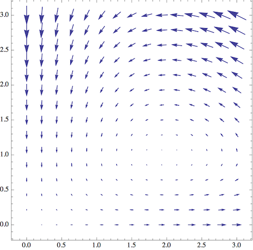
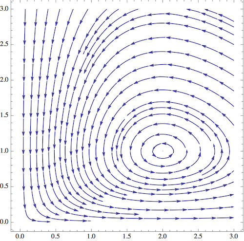
This is a very revealing picture! First of all, close to the axes, the derivatives follow the behavior that we predicted; the number of foxes is driven to be very small, and then the number of rabbits becomes very large. But the more interesting part of the diagram is near the equilibrium point \( (2,1) \). If I start nearby and follow the vector field around, the system seems to exhibit periodic behavior; the state goes around the equilibrium point in a closed loop. (If I draw the diagram very carefully, say by solving numerically with a computer, I find that the loops are indeed closed.)
We can take one of these curves and draw what is happening to \( R \) and \( F \) separately, and we get something like this, say for a starting point of \( (R,F) = (2,1/2) \):
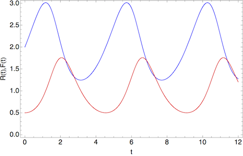
The population of rabbits is in blue, and that of foxes is in red. We see that the motion is periodic, although it's not described by sines and cosines (for other choices of initial values, the exponential nature of the growth and decay would be more obvious.) Note also that the population peak of foxes comes after the peak in rabbits; this is characteristic behavior of the Lotka-Volterra model.
It shouldn't surprise you to learn that there is actually a conserved quantity in this system, which does not change along any of these closed curves that we can draw. We can find it by noticing that if we multiply the first equation through by \( (c-dR)/R \), and the second equation by \( (a-bF)/F \), then the right-hand sides are equal and opposite, which means that
\[ \begin{aligned} \left( \frac{c}{R} - d \right) \dot{R} + \left( \frac{a}{F} - b \right) \dot{F} = 0. \end{aligned} \]
We can write this whole thing as one big time derivative:
\[ \begin{aligned} \frac{d}{dt} \left[ c \log R - dR + a \log F - bF \right] = 0. \end{aligned} \]
The quantity in brackets, which we call \( V \), is then always conserved: \( dV/dt = 0 \). So we can label any of the "orbits" we've seen by their values of \( V \). If we had done things in the opposite order, the existence of a conserved \( V \) would let us predict the closed curves we've been drawing (we can draw them parametrically in \( x \) and \( y \).)
Despite the fact that we can't write down an analytic solution, we can say a lot about the behavior of the Lotka-Volterra model, especially by drawing diagrams showing the orbits of the system. We'll make use of the same sorts of techniques to study physical systems; they will be particularly useful for the study of chaotic motion. But first we need to introduce some new formalism, that of Hamiltonian dynamics.