Since we just got back from break, let's warm up with a classic and simple example: the block on an inclined plane.
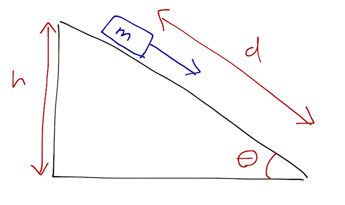
A block of mass \( m \) sits on a frictionless plane, inclined at angle \( \theta \). The block starts at rest with initial height \( h \), with \( d \) the displacement along the ramp from its starting point (so \( d = h / \sin \theta \) is the bottom of the ramp.)
Clicker Question
How long does the block take to reach the bottom?
A. \( t_f = \sqrt{\frac{2h}{g}} \sin \theta \)
B. \( t_f = \sqrt{\frac{2h}{g}} \frac{1}{\cos \theta} \)
C. \( t_f = \sqrt{\frac{2h}{g}} \frac{1}{\sin \theta} \)
D. \( t_f = \sqrt{2gh}\frac{1}{\sin \theta} \)
Answer: C
I'll go through the proper derivation below, but the real moral of this question is that all of the other options are obviously wrong - you only need to check units and limits! (Physicists always like to conserve energy when possible, so shortcuts are good.)
We can eliminate D first; \( h \) is a length and \( g \) an acceleration, so the units on the right hand side are \( \sqrt{m * (m/s^2)} = m/s \); this is a velocity, not a time. (Always, always, always check the units when solving a problem - you'll catch lots of algebraic mistakes that way!)
Next, consider the limit \( \theta \rightarrow 90^\circ \). In this limit the ramp no longer matters - the block is just in freefall. You may or may not remember that \( t_f = \sqrt{2h/g} \) is correct for an object in freefall, but you at least know answer B can't be right, because for \( \theta \rightarrow 90^\circ \) it gives infinite \( t_f \).
Finally, if we take \( \theta \rightarrow 0^\circ \), the block is sitting on a flat surface and doesn't move; it will never reach the bottom of the ramp. Since answer A gives \( t_f = 0 \), we can eliminate it, and the only choice left is C, which goes to infinity as \( \theta \rightarrow 0^\circ \) - as it should! (If you considered \( \theta \rightarrow 0^\circ \) first, you may have noticed that it also rules out choice B, which gives \( t_f = \sqrt{2h/g} \) and not infinity.)
(Note that I could have written any number of other solutions which are wrong, but still satisfy the checks we've gone through! Checking units and limits is a safety valve, not a solution method!)
If you did the solution properly, you did one of two things. You can write down a free-body diagram:
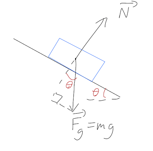
and then apply Newton's laws, balancing the forces in the normal direction:
\[ \begin{aligned} N = mg \cos \theta \\ F_{\textrm{net}} = m\ddot{d} = mg \sin \theta \end{aligned} \]
so with the block starting at rest, \( d = \frac{1}{2} (g \sin \theta) t^2 \). The block reaches the bottom when \( d = h / \sin \theta \), or
\[ \begin{aligned} t_f = \sqrt{\frac{2h}{g}} \frac{1}{\sin \theta}. \end{aligned} \]
We could have also used conservation of energy to do this in one line! We know that \( \Delta T = -\Delta U \), or
\[ \begin{aligned} (0 - \frac{1}{2} mv_f^2) = (mgh - 0) \\ v_f = \sqrt{2gh} \end{aligned} \]
Then, knowing that the block is experiencing constant acceleration, we know that \( v = at \), so \( d = \frac{1}{2} at_f^2 = \frac{1}{2} v_f t_f \), and therefore
\[ \begin{aligned} t_f = 2d / v_f = \frac{2(h/\sin \theta)}{\sqrt{2gh}} = \sqrt{\frac{2h}{g}} \frac{1}{\sin \theta}. \end{aligned} \]
We cheated a little with the energy approach here; we have to know something about the forces (and they have to be pretty simple!) for this method to work. I could have drawn any arbitrary shape for the ramp, and we still know \( v_f \), but to find the time taken we need to know the entire history of what the block did on its way down.
Of course, nothing is stopping us from solving this problem using Newton's laws, except that it will be quite complicated to keep track of the normal force along the ramp, since its direction is changing constantly. It would be great if we had a more general energy-based method, which would eliminate the need to keep track of such forces...
The brachistochrone problem
Let me ask a seemingly unrelated question about the ramp and block, which will lead us on a much needed mathematical detour. Suppose that instead of giving you a ramp, I give you the details of the block and the initial and final positions, and ask you to build a ramp which will minimize \( t_f \). How can you do it? (This is actually an old and famous problem in mechanics called the brachistochrone problem - Greek for "short time".)
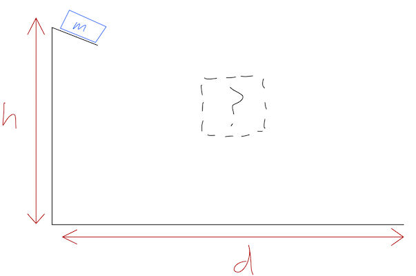
Let's be concrete: we can keep track of the position of our block as \( y(t) \), and we're given the two conditions
\[ \begin{aligned} y(0) = 0 \\ y(d) = -h. \end{aligned} \]
The shape of the ramp is some arbitrary function which we can write as \( y = f(x) \). Our only assumption will be that the ramp is well-behaved enough that the block doesn't get stuck somewhere in the middle before reaching \( x=d \).
The good news is that because this problem has only conservative forces, we can actually still use conservation of energy to solve it! We just have to be careful to account for the (unknown) shape of the ramp. At any instant, we know that \( T + U = 0 \) (since \( y(0)=0 \)), or
\[ \begin{aligned} T + U = 0 \\ \frac{1}{2} m (\dot{x}^2 + \dot{y}^2) + mgy = 0 \end{aligned} \]
Notice that although the presence of the ramp means that we don't have to keep track of \( x \) and \( y \) independently, the speed of the block still depends on both coordinates! We can rewrite:
\[ \begin{aligned} \dot{y} = \frac{dy}{dt} \\ = \frac{dy}{dx} \frac{dx}{dt} \\ = f'(x) \dot{x} \end{aligned} \]
where \( y' = df/dx \). Plugging back in above and rearranging:
\[ \begin{aligned} -2gy = \dot{x}^2 \left(1 + f'(x)^2 \right) \\ 1 = \frac{dx}{dt} \sqrt{ \frac{1+f'(x)^2}{-2gf(x)}} \\ t[f] = \int dt = \int_0^d dx \sqrt{ \frac{1+f'(x)^2}{-2gf(x)}}. \end{aligned} \]
That's our answer: given an arbitrary \( f(x) \), we can do the integral (at least numerically) to find the time taken for the block to reach the bottom. But we still haven't answered the main question: which \( f(x) \) will give us the optimal (i.e. fastest) \( t \)?
This is an example of an optimization problem, and we recall from calculus how to deal with them: the extreme (maximum and minimum) values of any function \( f(x) \) are found where its derivative vanishes. But \( t \) isn't a function of one variable, or even of a list of variables; it's a function of a function, \( f(x) \). Such an object is known as a functional.
A quick aside on a trick that I did above: I "split the derivative" by separating \( dx/dt \) and putting \( dt \) on the left side of the equation before integrating. This is something of an abuse of notation, although it's actually simple and rigorous if you don't skip steps. (If you are happy with Leibniz notation, i.e. thinking of separate "infinitesmals" \( dx \) and \( dt \), then splitting them apart is fine on its own.)
Here's how it works: if we have
\[ \begin{aligned} \frac{dx}{dt} f(x) = g(t) \end{aligned} \]
then we first integrate both sides with respect to \( t \),
\[ \begin{aligned} \int dt\ \frac{dx}{dt} f(x) = \int dt\ g(t). \end{aligned} \]
Now we just need to do a \( u \)-substitution on the left integral: if we change from \( dt \) to \( dx \), then
\[ \begin{aligned} \int \left[dx \frac{dt}{dx}\right] \frac{dx}{dt} f(x) = \int dt\ g(t), \end{aligned} \]
and we can cancel off \( dx/dt \) and its reciprocal, leaving the expression we would get from just splitting the derivative up,
\[ \begin{aligned} \int dx\ f(x) = \int dt\ g(t). \end{aligned} \]
Functionals
Just like a function is a map which takes some numbers as inputs and gives us a single number as output, a functional is a map from a function to a single number. Our solution to the ramp above is a functional: \( t[f] \) takes a function (the shape of the ramp) as input, and gives us a number (how long it takes to reach the bottom) as output.
Another very familiar functional is curve length, usually written \( S \). If we imagine drawing curves \( y(x) \) in the \( x-y \) plane, then for any such curve we can assign a length. If we break the curve down into infinitesmal pieces \( ds \), then we can write \( S \) as an integral:
\[ \begin{aligned} S[y] = \int_{y(x)} ds = \int_{y(x)} \sqrt{dx^2 + dy^2} \\ = \int dx\ \sqrt{1 + y'(x)^2} \end{aligned} \]
where \( y'(x) \equiv dy/dx. \)
(A brief note on notation: sometimes I like to put the \( dx \) on the left side of the integral, instead of the right. It means the same thing, not an integral times a function outside of it. I'll try to use brackets if things are ambiguous.
For every problem we will study in this class, the most general functional \( J \) acting on a single space of functions \( {y(x)} \) can always be written as an integral of the form
\[ \begin{aligned} J[y] = \int dx\ F(x, y, y'), \end{aligned} \]
where \( F \) is an ordinary function and again \( y' = dy/dx \). You can see that the examples we've studied so far both look like this. Now, you should be able to see where this is going: if we can define some version of a derivative on \( J[y] \), then maybe we can use it to solve the optimization problem.
Reminder: optimization in ordinary calculus
Before we do that, let's go back to single-variable calculus and remind ourselves of some details. What is the connection between on the derivative of a function that we use to locate the extrema (minimum and maximum points) of that function?
You can prove the relation using the definition of a derivative, which is probably what you did in math class, but another way is to use a Taylor series expansion. (In physics class, Taylor expansion should be the first tool you reach for in a lot of situations!) This second approach won't carry over directly to the calculus of variations, but it will help to give some intuition here.
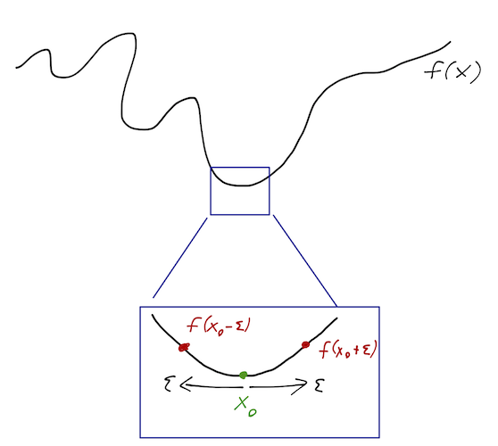
Recall that a Taylor series about the point \( x_0 \) is an infinite sum of increasing powers of \( (x-x_0)^n \). So if we're very close to \( x_0 \), we can just keep the first few terms and throw the rest away. Let's expand \( f(x_0 + \epsilon) \) about \( x_0 \):
\[ \begin{aligned} f(x_0 + \epsilon) = f(x_0) + \epsilon f'(x_0) + \frac{1}{2} \epsilon^2 f''(x_0) + ... \end{aligned} \]
Start by looking at the first term, \( \epsilon f'(x_0) \), which is linear in \( \epsilon \). This tells you if you zoom in far enough, the function \( f(x) \) itself looks linear at the point \( x_0 \). But that means that \( f(x) \) increases in one direction, and decreases in the other - it can't be an extreme value!
\[ \begin{aligned} f(x_0 + \epsilon) \approx f(x_0) + \epsilon f'(x_0) \\ f(x_0 - \epsilon) \approx f(x_0) - \epsilon f'(x_0) \end{aligned} \]
The only way out is for this term to vanish, so once again we're lead to the necessary condition \( f'(x_0) = 0 \).
Now suppose the first term is zero, and look at the second term. This term is quadratic in \( \epsilon \) - locally, \( f(x) \) looks like a parabola. So the sign of \( f''(x_0) \) matters - it tells us whether the parabola opens up (minimum) or down (maximum). Hence, testing the sign of the second derivative lets us decide whether we have a minimum or maximum.
Clicker Question
If \(f'(x_0) = 0\) and \(f''(x_0) = 0\), what do we know about the point \(x_0\)?
A. \( x_0 \) is a local minimum of \( f(x) \).
B. \( x_0 \) is a local maximum of \( f(x) \).
C. \( x_0 \) is a saddle point of \( f(x) \) - neither minimum nor maximum.
D. One of the above is true, it depends on the higher derivatives at \( x_0 \).
Answer: D
(Note: we skipped this clicker question due to time, and just discussed it as a class instead.)
When both terms vanish, we need to keep going in the Taylor series, calculating higher derivatives until we discover whether \( f(x) \) is locally even or odd around the point \( x_0 \). (Think of \( f(x) = x^n \) at \( x_0=0 \). \( x^3 \) has a saddle point there, but \( x^4 \) has a local minimum!)
Next time: calculus of variations!