Last time, we were discussing optimization problems. We reviewed how this works in ordinary calculus a bit, finding extrema of a function by looking at derivatives. But the more interesting optimization problems involve functionals, which are functions of functions. The example we saw was the brachistochrone problem, where we want to optimize \( t[y] \), the time it takes for a block to slide down a ramp of unknown shape \( y(x) \). Another common functional optimization problem is finding the shortest distance between two points, which involves the path length \( S[y] \).
To define a functional, we also have to define the space of functions on which it acts. If we want to use \( S \) to ask the question "what is the shortest distance between point A and point B in the plane?", then we would restrict \( {y(x)} \) to all functions \( y(x) \) that begin and end at those points. We had a similar restriction on the endpoints in our brachistochrone problem.
Let's be explicit and do a quick, concrete comparison between "function" and "functional". Take as an example the function
\[ \begin{aligned} y(x) = 3x^2. \end{aligned} \]
The simplest thing we can do with a function is to evaluate it, i.e. to ask the question "what is \( y(x) \) at \( x=1 \)?" Optimization problems ask the more difficult question "at which value of \( x \) is \( y(x) \) [minimum/maximum]?", which requires us to evaluate \( y'(x) \) and solve for where it vanishes (and to look at higher derivatives, usually.)
Now let's look at the functional version of all of the above. We can define a simple functional as the area under a curve from 0 to 1:
\[ \begin{aligned} A[y(x)] = \int_0^1 dx\ y(x). \end{aligned} \]
We are implicitly fixing boundary conditions when we define this functional; there is some set of functions \( y(x) \) we're willing to consider. Let's say in this case we want to fix \( y(0) = 0 \) and \( y(1) = 3 \), so that \( 3x^2 \) is one example. Now, the simplest thing we can do with \( A \) is evaluate it at a specific function: "What is \( A[y(x)] \) with \( y(x) = 3x^2 \)?" We can also optimize, i.e. "What is the function \( y(x) \) (with the given boundary conditions) which minimizes (or maximizes) \( A[y] \)?"
What does an extreme (minimum or maximum) function look like, given some functional? If \( y_0(x) \) is a minimum of \( A[y] \), we expect that if we "move away" from \( y_0(x) \) just a little bit, if we adjust some part of the curve, we will always find that our new \( y(x) \) satisfies \( A[y] > A[y_0] \).
The general problem, Euler's equation
Okay, let's get back to our more general variational problem setup, with the definition of our general functional \( J \):
\[ \begin{aligned} J[y] = \int_a^b dx\ F(x, y, y'). \end{aligned} \]
To decide whether the functional \( J[y] \) is at an extremum for some given curve \( y_0(x) \), we need a sensible way to compare \( y_0(x) \) to "nearby" curves in the same class. How do we decide what "nearby" means for a curve? We can construct such a nearby curve like so:
\[ \begin{aligned} y(x) \equiv y_0(x) + \alpha \eta(x) \end{aligned} \]
where \( \alpha \) is a real number, and \( \eta(x) \) is some other smooth curve. So long as \( \eta(x) \) is well-behaved, we can always ensure \( y(x) \) is "near" to \( y_0(x) \) by making \( \alpha \) sufficiently small.
Note that implicit in writing \( J[y] \) is a choice of boundary conditions; the functional isn't defined properly without them! This means that not only are we fixing the range of integration from \( x=a \) to \( x=b \), but we're only considering functions which satisfy some conditions
\[ \begin{aligned} y(a) = y_1 \\ y(b) = y_2 \end{aligned} \]
Fixing the endpoints is very important; it means that when we write the "nearby" function in the sketch as
\[ \begin{aligned} y(x) = y_0(x) + \alpha \eta(x), \end{aligned} \]
the difference between them satisfies
\[ \begin{aligned} \eta(a) = \eta(b) = 0. \end{aligned} \]
This will be important in our proof, and more generally it's needed so that we have a well-defined problem to solve. (Going back to the path length, you can ask the question "what is the shortest curve between two points", but the question "what is the shortest curve" doesn't make much sense.) Here's a sketch of our setup:
![Setup for studying extreme points of a functional \\( J[y] \\).](https://physicscourses.colorado.edu/phys3210/phys3210_sp20/images/fig-variation.png)
(Note that I'm not defining the quantity \( \epsilon \), but if we want to be more careful mathematically we could - clearly by adjusting \( \alpha \) we can make the envelope \( \epsilon \) bounding the difference between functions arbitrarily small.)
We can expand out the functional value of this nearby curve:
\[ \begin{aligned} J[y] = \int_a^b dx\ F(x, y_0+\alpha \eta, y_0' + \alpha \eta') \\ \Delta J \equiv J[y] - J[y_0] = \int_a^b dx\ \left( F(x,y_0+\alpha \eta, y_0' + \alpha \eta') - F(x,y_0,y_0') \right). \end{aligned} \]
Because \( \alpha \) can be made infinitesmally small, we can Taylor expand \( F \) around our original function \( y_0 \). (If this seems like a suspicious thing to do, you can think about doing the expansion given a fixed value of \( x \); since our argument will carry through no matter what \( x \) is, there's no problem with applying Taylor's theorem under the integral here.) Expanding to first order, we have for a multivariate function
\[ \begin{aligned} f(x+\epsilon,y) = f(x,y) + \epsilon \frac{\partial f}{\partial x}(x,y) + ... \end{aligned} \]
(which is just the one-variable version since we're holding \( y \) fixed), so in the functional above,
\[ \begin{aligned} \Delta J = \int_a^b dx\ \left( \frac{\partial F}{\partial y} \alpha \eta(x) + \frac{\partial F}{\partial y'} \alpha \eta'(x) \right) \\ \end{aligned} \]
Just as for ordinary functions, it turns out that the condition for \( J[y_0] \) to be a minimum is that the infinitesmal difference between \(J[y_0]\) and the nearby curve \( J[y] \) should go to zero as \( \alpha \) does: \( \lim_{\alpha \rightarrow 0} \Delta J / \alpha = 0 \), or \( dJ/d\alpha = 0 \) if you prefer. The difference now is that we have an arbitrary function \( \eta(x) \) as well, and the difference should vanish for any choice of \( \eta \).
Let's try to simplify this: since \( \eta \) is arbitrary we don't know how \( \eta \) and \( \eta' \) are related, but we can still integrate by parts to move the derivative off of \( \eta' \):
\[ \begin{aligned} \int_a^b dx\ \frac{\partial F}{\partial y'} \alpha \eta'(x) = \left.\alpha \eta(x) \frac{\partial F}{\partial y'}\right|_a^b - \int_a^b dx\ \alpha \eta(x) \frac{d}{dx} \left(\frac{\partial F}{\partial y'}\right). \end{aligned} \]
Importantly, the boundary term vanishes by construction, since \( \eta(a) = \eta(b) = 0 \)! So we can combine the other two terms under the integral, which are now both proportional to \( \eta \):
\[ \begin{aligned} \Delta J = \int_a^b dx\ \alpha \eta(x) \left[ \frac{\partial F}{\partial y} - \frac{d}{dx}\left(\frac{\partial F}{\partial y'}\right) \right]. \end{aligned} \]
Note that the connection to extreme values of \( J[y] \) is easy to see! If \( y_0 \) is a minimum of \( J[y] \), then we must have \( \Delta J \geq 0 \). But this first term is, in a sense, linear in the variation \( \eta(x) \). If the integral gives us any positive number, then the same integral with \( \eta \rightarrow -\eta \) will be negative, contradicting the statement that \( y_0 \) is a minimum. So the only possibility is that the integral vanishes.
This doesn't mean that all of \( \Delta J \) vanishes; there are still higher-order terms, remember. But in many books you will see a special notation for this first term. Given a functional \( J[y] \), we write
\[ \begin{aligned} \delta J \equiv \int dx\ \delta y \left[\frac{\partial F}{\partial y} - \frac{d}{dx}\left(\frac{\partial F}{\partial y'}\right)\right]. \end{aligned} \]
\( \delta J \) is called the variation of the functional, and \( \delta y \) (which was \( \alpha \eta \), but I've changed it to more conventional notation) is called the variation of the curve \( y(x) \). The condition for a minimum or maximum is then
\[ \begin{aligned} \delta J = 0. \end{aligned} \]
The variation \( \delta J \) is essentially the equivalent of the first derivative for a functional. You might be tempted to try to write the expression in square brackets as something like \( \delta J / \delta y \), but remember that \( \delta y \) is a function of \( x \); you can't move it outside the integral. From the condition that \( \delta J = 0 \), which has to hold for any \( \delta y \), we arrive at the celebrated Euler-Lagrange equation:
(Euler-Lagrange equation)
\[ \begin{aligned} \frac{\partial F}{\partial y} - \frac{d}{d x}\left(\frac{\partial F}{\partial y'}\right) = 0. \end{aligned} \]
Any curve \( y \) satisfying the Euler-Lagrange (sometimes written E-L for short) equation gives a stationary point of the functional \( J[y] \) (defined as an integral over \( F \) as we have done.)
I've done all of this for only one dependent variable, but if we have more than one dependent variable \( y_1, y_2, ... \), the functional becomes
\[ \begin{aligned} J = \int dx\ F(x, y_1, y_1', y_2, y_2', ...) \end{aligned} \]
and the total variation just becomes a sum over the same integral expression for each variable - in other words, we do the same derivation for one \( y \) at a time. Thus, the generalization to multiple dependent variables is just that we get a system of Euler-Lagrange equations instead,
\[ \begin{aligned} \frac{\partial F}{\partial y_i} - \frac{d}{dx}\left(\frac{\partial F}{\partial y_i'}\right) = 0. \end{aligned} \]
The book has some additional detail on this. This multiple-variable form will be extremely useful when we get back to mechanics, when we'll want to keep track of complicated systems that have multiple objects with different coordinates.
Example: shortest distance between two points on a plane
Back to our shortest-distance problem. We wrote the curve-length functional already,
\[ \begin{aligned} S = \int_a^b dx\ \sqrt{1 + y'^2}. \end{aligned} \]
Taking derivatives of the integrand:
\[ \begin{aligned} \frac{\partial F}{\partial y} = 0, \\ \frac{\partial F}{\partial y'} = \frac{y'}{\sqrt{1+y'^2}}. \end{aligned} \]
The E-L equation is thus
\[ \begin{aligned} \frac{\partial}{\partial x}\left( \frac{y'}{\sqrt{1+y'^2}} \right) = 0. \end{aligned} \]
Expanding the derivative out would make life more complicated; instead we use the knowledge that the left-hand side is constant with respect to \( x \), so
\[ \begin{aligned} y' = C\sqrt{1+y'^2} \end{aligned} \]
for some number \( C \). Squaring and rearranging, this means that
\[ \begin{aligned} y'^2 = C^2 (1 + y'^2) \\ y'^2 = \frac{C^2}{1-C^2}. \end{aligned} \]
or \( y' = m \), for some other constant \( m \)! This is a very simple differential equation, which we can solve by just integrating both sides, giving:
\[ \begin{aligned} y(x) = mx + c \end{aligned} \]
which is, of course, a straight line. We could now solve for \( m \) and \( c \) in terms of the endpoints by using the boundary conditions if we wanted.
Notice that our solution of the E-L equation simplified here, because \( F \) didn't depend on \( y \), just \( y' \). For \( F \) independent of \( y' \), the E-L equation is even simpler - we just get \( \partial F / \partial y = 0 \). Finally, if \( F \) is independent of \( x \), we can also write down a simplified version of the E-L equation (you'll derive this in the homework):
\[ \begin{aligned} \frac{\partial F}{\partial x} = 0 \Rightarrow F - y' \frac{\partial F}{\partial y'} = \textrm{const.} \end{aligned} \]
This is sometimes called the second form of the Euler-Lagrange equation, and it can simplify certain problems.
Example: shortest distance between two points on a sphere
Let's do a more interesting shortest-distance problem. (Math aside: the shortest distance connecting two points on a general surface is called a geodesic.) Obviously we should use spherical coordinates! If you start with \( ds = \sqrt{dx^2 + dy^2 + dz^2} \) and change coordinates, you will find:
\[ \begin{aligned} ds^2 = dr^2 + r^2 d\theta^2 + r^2 \sin^2 \theta d\phi^2. \end{aligned} \]
Letting \( R \) be the radius of the sphere, \( dr \) vanishes since we're moving on the surface, and so
\[ \begin{aligned} S = \int \sqrt{R^2 d\theta^2 + R^2 \sin^2 \theta d\phi^2} \\ = R \int_{\theta_a}^{\theta_b} d\theta\ \sqrt{ 1 + \phi'(\theta)^2 \sin^2 \theta}. \end{aligned} \]
Since \( F(\theta, \phi, \phi') \) doesn't depend on \( \phi \), the Euler-Lagrange equation simplifies to
\[ \begin{aligned} \frac{\partial F}{\partial \phi'} = C \\ \frac{\sin^2 \theta\ \phi'}{\sqrt{1 + \sin^2 \theta\ \phi'^2}} = C. \end{aligned} \]
At this point we can solve for \( \phi' \) and then integrate over \( \theta \), but finding the solution and then interpreting the result is sort of messy. Instead, we can exploit the symmetry of the sphere. We want the path from point \( A \) to point \( B \), but we can rotate the sphere around to put point \( A \) where we want. The best place to put it is at the north pole, \( \theta_A = 0 \), which immediately gives us \( C = 0 \). But if \( C \) vanishes for the entire trajectory, then we must have
\[ \begin{aligned} \frac{d\phi}{d\theta}= 0. \end{aligned} \]
So the shortest path is a line of longitude, with the sphere rotated to this orientation. More generally, if we rotate the sphere again the path becomes a great circle, which is the intersection of a plane through the center of the sphere with the sphere itself.
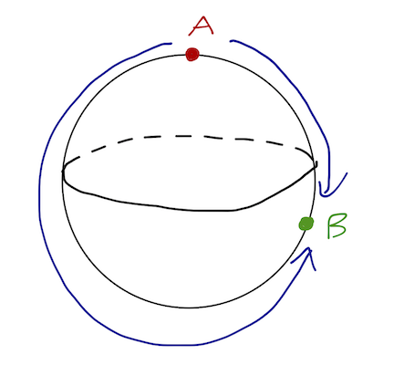
Notice that there are two paths satisfying the E-L equation, clockwise or counter-clockwise. (If you're flying from Denver to New York, you can go east or west, for example.) The shorter path of the two is the true minimum distance.
Clicker Question
Which is true of the longer route from \( A \) to \( B \)? (Ignore the special case where the length of the "long" and "short" routes is equal.)
A. It is not a valid solution; it does not satisfy the E-L boundary conditions.
B. It (locally) maximizes the path length.
C. It is a saddle point of the path length.
D. It (locally) minimizes the path length.
Answer: C
The solution is valid; the E-L boundary conditions are satisfied since it is a path from point \( A \) to point \( B \). We can also discard the possibility of a local maximum, because given any path on a sphere, it's really easy to make a longer one, say by circling around the sphere a few times before arriving at \( B \). (In fact, there is no maximum path length, if you think about it.)
This leaves either a local minimum, or a saddle point. The definition of a saddle point is that there should be some ways in which we can deform the curve to make it longer, and other ways to make it shorter. There are lots of ways to make the curve longer - imagine a path that oscillates around the drawn path, for example. But we can also make it shorter: imagine "pushing" the long path towards the shorter one along the surface of the sphere. This deformed path is no longer an Euler-Lagrange equation solution, but it is shorter!
Even in this relatively simple example, we had to worry about what sort of stationary points solving the Euler-Lagrange equation gave us! But don't worry too much - for most physical problems we will deal with, the functional will have a minimum but no maximum value (just like the path length.) This means that in most situations the minimum solution will exist and be unique. For those special cases like the sphere where saddle points may also appear, we can figure out which one is the minimum just by testing which solution gives the smallest value of the functional.
Next time: back to mechanics!