Last time, we finished up our study of calculus of variations and did a couple of examples. Now let's go back and finally solve the problem that I used to motivate the calculus of variations in the first place.
Example: the brachistochrone problem
(Note: I didn't go through this solution in detail in lecture, because it's a little cumbersome, and requires a very non-obvious solution to evaluate the integral near the end. I'm leaving the full details here for the curious.)
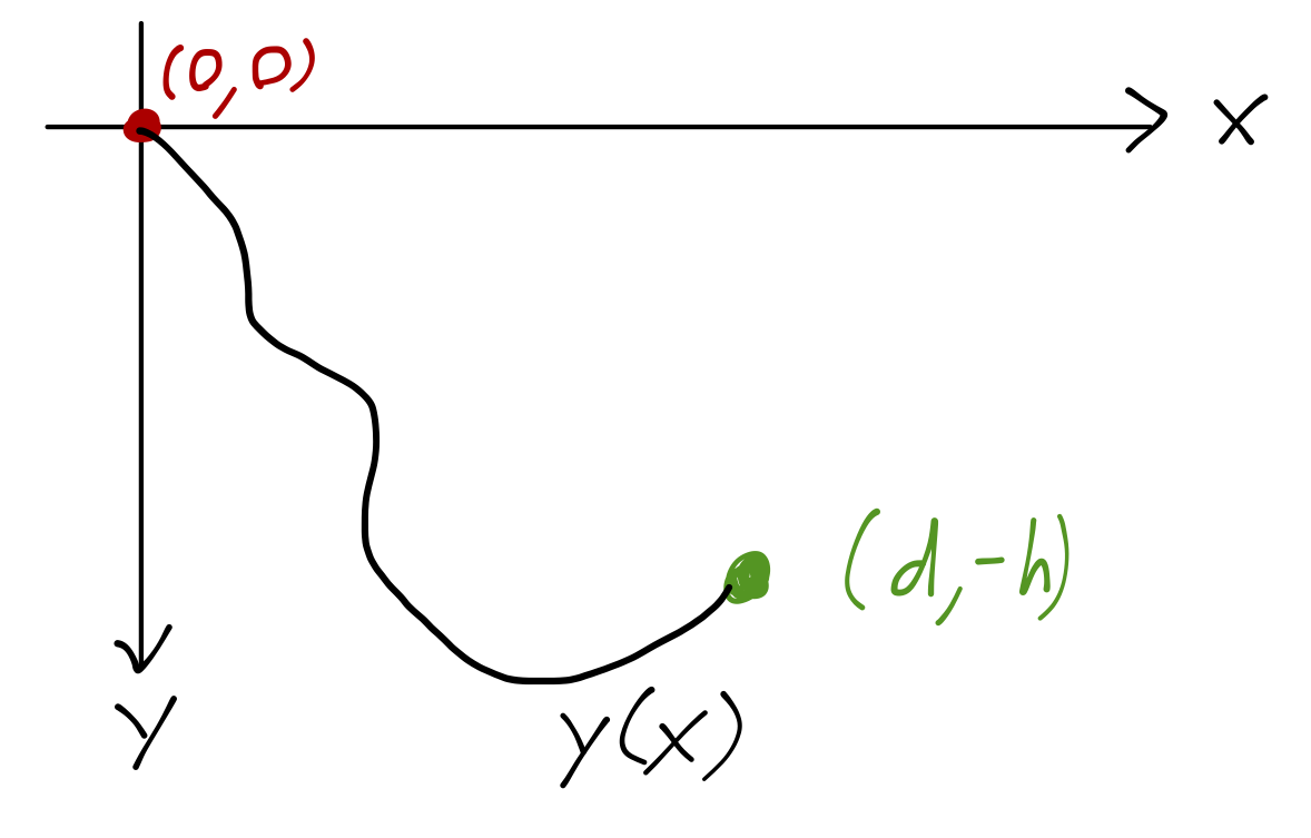
Once again, the problem involves letting the shape of the ramp be arbitrary: we have to optimize over the time taken for the block to reach the bottom. As before I keep the height \( h \) and distance \( d \) to the final point fixed. In fact, let me fix a coordinate system: let's take \( y(0) = 0 \) and \( y(d) = -h \). We are interested in finding \( y(x) \) which minimizes the time for our block to reach the bottom. This is a very famous problem in physics, known as the brachistochrone (from the Greek words for "short time".)
Since the ramp is frictionless, we know that \( v = \sqrt{-2gy} \) by conservation of energy. So, the time functional is:
\[ \begin{aligned} t = \int dt = \int \frac{ds}{v} \\ = \int \frac{\sqrt{dx^2 + dy^2}}{\sqrt{-2gy}} \\ = \int_{-h}^0 dy\ \sqrt{\frac{x'^2 + 1}{-2gy}}. \end{aligned} \]
We've used \( x \) as the dependent variable, so the E-L equation simplifies:
\[ \begin{aligned} \frac{\partial F}{\partial x'} = C = \frac{x'}{\sqrt{y(x'^2+1)}} \\ C^2 y (x'^2 + 1) = x'^2 \\ x'^2 = \frac{C^2 y}{1 - C^2 y} \\ \frac{dx}{dy} = \sqrt{\frac{y}{2a - y}} \end{aligned} \]
where \( a \) is a new constant that we've chosen to give a nice-looking final answer. We can do a sneaky substitution to integrate and solve this diff. eq! Let \( y = a(1 - \cos \theta) \), so that \( dy = d\theta\ a \sin \theta \). Then the integral for \( x \) simplifies drastically:
\[ \begin{aligned} x = \int dy\ \frac{\sqrt{1 - \cos \theta}}{\sqrt{1+\cos \theta}} \\ = \int dy\ \frac{1-\cos \theta}{\sqrt{1-\cos^2 \theta}} \\ = \int (d\theta\ a \sin \theta) \frac{1-\cos \theta}{\sin \theta} \\ = a (\theta - \sin \theta) + x_0. \end{aligned} \]
So we now have a parametric solution for the path - \( x \) as above, and \( y(\theta) = a(1-\cos \theta) \). Since our boundary values for \( y \) are \( h \) and \( 0 \), we can identify \( x(\theta=0) = y(\theta=0) = 0 \), fixing \( x_0 = 0 \). At the other end, we have the system of equations
\[ \begin{aligned} x(\theta_f) = d = a(\theta_f - \sin \theta_f)\\ y(\theta_f) = -h = a(1-\cos \theta_f) \end{aligned} \]
Inverting for \( a \) and \( \theta_f \) is messy; for most cases, you can only do it numerically. However, we can draw the general parametric curve to give you some idea of what solutions look like in general:
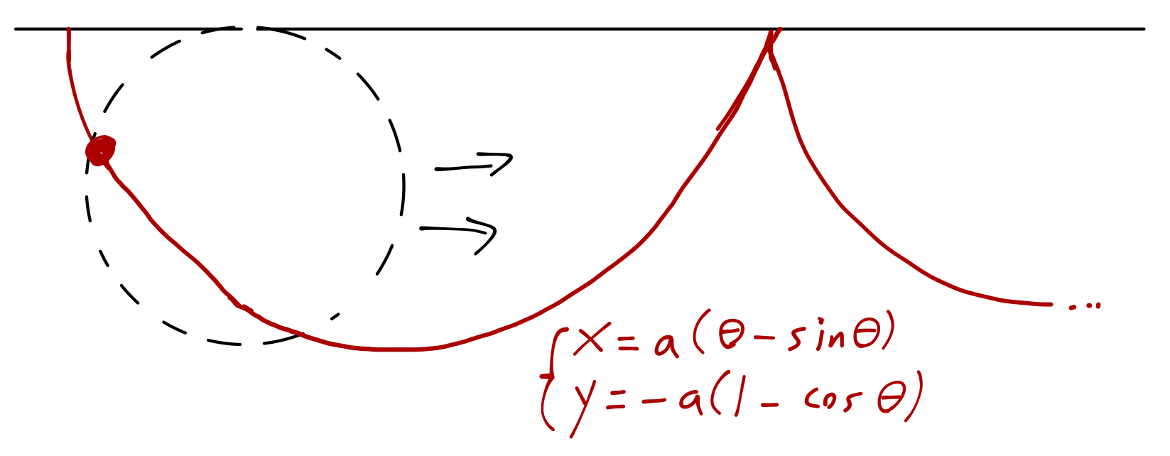
This curve is known as a cycloid (or sometimes as a brachistochrone) - it is the curve traced by point on a circle rolling along the \( x \)-axis. Note that depending on the values of \( d \) and \( h \), the fastest path can actually overshoot and come back up to the endpoint.
The cycloid result seems a little counterintuitive, so it's nice to see it in action. Unfortunately, when I've tried doing a demo of this in the past, it's pretty hard to really see the outcome. Fortunately, the internet exists! Here's a video of Adam Savage demonstrating a brachistochrone against a couple of other ramp shapes, and here's the full video of its construction.
Back to classical mechanics: the Lagrangian
So, how does all of this relatively esoteric math about optimization problems help us to solve general problems in classical mechanics? If I take us all the way back to our starting example of the fixed ramp and the block:
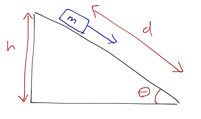
there doesn't appear to be anything to optimize here. With a complete initial condition as sketched here, we know that classical mechanics is deterministic; Newton's laws will tell us how the system evolves at any instant in time, and the evolution of the system is completely fixed. How would calculus of variations even show up here?
Let's try to look at the system in a different way. When we solve for the motion of the block, we are finding the function \( y(t) \) that describes its position as a function of time. (The presence of the ramp means if we know \( y \), we know \( x \) too.) In a sense, then, we can think of the correct solution as a "path" through space and time:
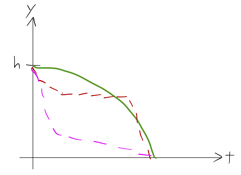
Newton's laws tell us that the block will follow the solid path, and not any of the dotted ones: it won't come to a stop and then start again, or accelerate rapidly and then move at constant speed. Our solution is a single "path" out of many possibilities we could have imagined. But if classical mechanics is really optimizing over paths like this, then what is the functional that's being optimized?
Taylor just sort of throws the answer to this mystery at you, but in fact we can find a strong hint hidden in Newton's laws if we stare at them long enough. Let's see if we can guess the right functional to use, starting with a simple example, namely a single particle of mass \( m \) moving in one dimension \( x \).
Newton's second law is then
\[ \begin{aligned} F = m\ddot{x}. \end{aligned} \]
(Quick reminder of notation: dots are special notation for time derivatives, so \( \dot{x} = dx/dt \), and \( \ddot{x} \) is the second derivative.)
To go further, we have to assume something about \( F \). Recall from last semester that many forces are conservative, and that conservative forces have some nice properties. A conservative force is one which conserves mechanical energy: if a particle in a conservative force field comes back to where it started, no work will have been done on it. This means that we can write a potential energy function \( U \), the gradient of which gives the force field:
\[ \begin{aligned} \vec{F} = -\nabla U \end{aligned} \]
or for our one-dimensional example, \( F = -dU/dx \). So Newton's law becomes
\[ \begin{aligned} m \ddot{x} = -\frac{dU}{dx}. \end{aligned} \]
This still doesn't look much like anything we would get from an Euler-Lagrange equation. But as long as we're writing down energy functions, let's recall what the kinetic energy \( T \) of our particle looks like:
\[ \begin{aligned} T = \frac{1}{2} m \dot{x}^2. \end{aligned} \]
Since lately we've been thinking in terms of taking partial derivatives with respect to other derivatives, if you stare at this for awhile, you'll notice that the derivative of \( T \) is particularly simple:
\[ \begin{aligned} \frac{\partial T}{\partial \dot{x}} = m \dot{x}. \end{aligned} \]
This is just one time derivative from being the left-hand side of Newton's law!
\[ \begin{aligned} \frac{d}{dt} \left( \frac{\partial T}{\partial \dot{x}}\right) = m\ddot{x}, \end{aligned} \]
so
\[ \begin{aligned} \frac{\partial U}{\partial x} + \frac{d}{dt} \left( \frac{\partial T}{\partial \dot{x}} \right) = 0. \end{aligned} \]
This almost looks like an Euler-Lagrange equation, except that one term is acting on \( U \), and the other on \( T \). But notice that \( U \) doesn't depend on the velocity \( \dot{x} \), and \( T \) doesn't depend on the position \( x \). So if we combine the two into a quantity called the Lagrangian:
(The Lagrangian)
\[ \begin{aligned} \mathcal{L} \equiv T - U \end{aligned} \]
then the motion of our particle does satisfy an Euler-Lagrange equation,
\[ \begin{aligned} \frac{\partial \mathcal{L}}{\partial x} - \frac{d}{dt} \left( \frac{\partial \mathcal{L}}{\partial \dot{x}}\right) = 0. \end{aligned} \]
The functional that is minimized by the solution of this equation is the integral of the Lagrangian, and it is called the action:
(Action)
\[ \begin{aligned} S = \int_{t_i}^{t_f} dt\ \mathcal{L}(t,x,\dot{x}). \end{aligned} \]
So (for a conservative force, and with no further constraints), we have shown that applying Newton's laws and solving for the motion of a test particle is equivalent to solving for the path for which the action \( S \) is stationary, i.e. where the first variation \( \delta S \) (which we defined last week) vanishes,
(Hamilton's principle)
\[ \begin{aligned} \delta S = 0. \end{aligned} \]
Notice that the Lagrangian has units of energy, by definition. The integral is over time, so the units are energy * time. Unfortunately, unlike energy or momentum which are physical quantities you have some intuition for, there's not really a good, intuitive way to think about what the action means - at least not in classical mechanics. (Just as a teaser, you might remember that you've seen one physical constant with units of action before, in your modern physics class: Planck's constant, \( h \).)
Lagrangian Mechanics
Now that we've seen the basic statement, let's begin to study how we apply the Lagrangian to solve mechanics problems.
Because this is new and strange, I'll stress once again that this is a reformulation of classical mechanics as you've been learning it last semester; it's just a different way of obtaining the same physics. Hamilton's principle implies Newton's laws, and Newton's laws imply Hamilton's principle. What we have shown is that, for a mechanical system being acted on by only conservative forces \( \vec{F} \), there are three statements we can make which are all completely equivalent to each other:
- The system evolves under Newton's laws, \( \vec{F} = m\ddot{\vec{r}} \) (etc.)
- The particle travels along a path for which the action is stationary, \( \delta S = 0 \).
- The particle travels along a path determined by the Euler-Lagrange equations,
\[ \begin{aligned} \frac{\partial \mathcal{L}}{\partial x_i} - \frac{d}{dt}\left(\frac{\partial \mathcal{L}}{\partial \dot{x_i}}\right) = 0. \end{aligned} \]
Requiring conservative forces might seem like a strong restriction; we can't deal with friction, or air resistance, for example. But there will be plenty of interesting cases that we can treat using the Lagrangian. (It is actually possible to deal with these effects in a Lagrangian framework, but it's much more complicated so we won't do it here.)
Moreover, there is something deeply fundamental about the action and Hamilton's principle, as I mentioned. You will see it again and again in your physics classes; in electromagnetism, and especially in quantum mechanics. At the microscopic level, all of the fundamental forces that we know of are conservative, so in principle there is no system that the Lagrangian approach can't be applied to. Non-conservative forces like friction are a sort of bookkeeping trick, since we can't possibly deal with keeping track of all of the interactions between molecules happening as a block slides down a ramp. Energy isn't really being lost for good due to friction, it's just disappearing into part of the system that we're not keeping track of.
Clicker question
A particle moves in one dimension \( x \), with Lagrangian \( \mathcal{L} = T - U \). Suppose we shift the potential energy definition \( U \) by a constant \( C \). What changes?
A. Nothing happens; the action and the physical path \( x(t) \) do not change.
B. The value of \( S \) changes, but the path \( x(t) \) which gives \( \delta S = 0 \) does not.
C. The new physical path \( x(t) \) is found by solving the equation \( \delta S = C \).
D. The old physical path is shifted to \( x_{\textrm{new}}(t) = x_{\textrm{old}}(t) + C \).
Answer: B
Shifting \( U \) by a constant has no effect on the physical path! (You already knew this was true from Newtonian mechanics, of course.) The Euler-Lagrange equations only involve derivatives of the Lagrangian, so they do not change when a constant shift is added. However, our shift does change the action, which is the integral of \( \mathcal{L} = T-U \), by the value \( \Delta S = C(t_f - t_i) \).
(Note: the way this was phrased, it was a little unclear that I intended to keep the boundary conditions fixed. However, in the lab there's another way to shift the potential energy: if our particle is moving under gravity, we can just shift the position of the particle to change the potential by a constant. This would trivially change the physical path by a constant. Due to the ambiguity, I'll count D as a correct answer here - although on dimensional grounds, it can't be the same constant \( C \) shifting \( U \) and \( x \)!)
We spent some time worrying last week about minima vs. maxima vs. saddle points, and in fact Hamilton's principle is sometimes called the principle of least action, but note that the condition here is just that we find a stationary point. It's not at all obvious why only a stationary point is good enough - I may say a few words about that at the very end of the semester, leading in to quantum mechanics.
You might be puzzled that we ended up with this strange new object \( S \) to minimize over, instead of simply the total energy \( E = T + U \). But minimizing the total energy doesn't give us the solution corresponding to Newton's laws, while minimizing the action does, as we just proved.